MultivAreate
This blogpost will introduce the core of MultivAreate, a statistical model for (areal) typology and dialectology. If you find this tutorial useful please cite:
Guzmán Naranjo, Matías and Mertner, Miri. “Estimating areal effects in typology: a case study of African phoneme inventories” Linguistic Typology, vol. 27, no. 2, 2023, pp. 455-480. https://doi.org/10.1515/lingty-2022-0037
Introduction
A problem often encountered in typology and dialectology is how to handle multiple (binary) outcomes at the same time. Imagine, for example, we are interested in modelling the distribution of different phonemes: /p/, /t/, /k/, etc. and we want to predict the presence or absence of each phoneme from some covariate X, or maybe we are just interested in the overall distribution of these phonemes in space, or want to know, after cotrolling for a series of confounds, which phoneme is most frequent.
An initial idea would be to model each phoneme independently of each other in some type of logistic regression (in R notation): \(/p/ \sim 1 + x1 + x2 + …\). The problem emerges because we know (or at least suspect) that our different dependent variables (presence of /p/, /t/, /k/, etc.) are correlated, but by modelling them as independent we are ignoring this correlation structure. Additionally, there are cases in which we might have some predictior \(x_i\) which is shared across multiple outcomes. This type of situation is not possible to capture with independent models.
What we want is a model that allows us to capture multiple binary outcomes, simultaneously, and as correlated.
Correlated continuous outcomes
Before moving to binary outcomes, I will quickly go over something much simpler: correlated continuous outcomes. We will start by using some synthetic data.
library(mvtnorm)
library(rstan)
## Loading required package: StanHeaders
##
## rstan version 2.32.6 (Stan version 2.32.2)
## For execution on a local, multicore CPU with excess RAM we recommend calling
## options(mc.cores = parallel::detectCores()).
## To avoid recompilation of unchanged Stan programs, we recommend calling
## rstan_options(auto_write = TRUE)
## For within-chain threading using `reduce_sum()` or `map_rect()` Stan functions,
## change `threads_per_chain` option:
## rstan_options(threads_per_chain = 1)
library(tidyverse)
## ── Attaching core tidyverse packages ───────────────────────────────────────────────── tidyverse 2.0.0 ──
## ✔ dplyr     1.1.4     ✔ readr     2.1.5
## ✔ forcats   1.0.0     ✔ stringr   1.5.1
## ✔ ggplot2   3.5.1     ✔ tibble    3.2.1
## ✔ lubridate 1.9.3     ✔ tidyr     1.3.1
## ✔ purrr     1.0.2
## ── Conflicts ─────────────────────────────────────────────────────────────────── tidyverse_conflicts() ──
## ✖ tidyr::extract() masks rstan::extract()
## ✖ dplyr::filter()  masks stats::filter()
## ✖ dplyr::lag()     masks stats::lag()
## ℹ Use the conflicted package (<http://conflicted.r-lib.org/>) to force all conflicts to become errors
library(ape)
##
## Attaching package: 'ape'
##
## The following object is masked from 'package:dplyr':
##
##     where
library(geodist)
library(parallel)
library(rnaturalearth)
library(sf)
## Linking to GEOS 3.12.2, GDAL 3.9.1, PROJ 9.4.1; sf_use_s2() is TRUE
## devtools::install_github('Mikata-Project/ggthemr')
library(ggthemr)
ggthemr("fresh")

mu <- c(2, 3)
rho <- 0.3
Sigma <- diag(2) * (1 - rho) + rho
set.seed(1234)
Y <- rmvnorm(100, mean = mu, sigma = Sigma)
Here we have generated two correlated random variables with means \(2\) and \(3\), sd = \(1\) and a correlation of \(0.3\). We can test the empirical correlation very easily.
round(cor(Y), 2)
##      [,1] [,2]
## [1,] 1.00 0.36
## [2,] 0.36 1.00
Which ends up being \(0.36\), close enough to the \(0.3\) assigned to rho. And the effectively the means.
round(colMeans(Y), 2)
## [1] 1.99 2.88
Now, imagine we want to capture this data. The stan model is simple enough. We model Y, the dependent variable, as coming from a multivariate normal distribution with means on the paramenter intercept and Sigma equal to diag(sigma) %*% rho %*% diag(sigma) where rho is the correlation matrix.
We can fit this model as follows.
model_1 <- "data {
  int N; // number of rows (observations)
  int K; // number of columns (variables)
  array[N] vector[K] Y;
}
parameters {
  vector[K] intercept;  // intercepts
  corr_matrix[K] rho;   // correlation factor
  vector<lower=0>[K] sigma; // sigma
}
model {
  rho   ~ lkj_corr(2);       // generic prior on the correlation
  sigma ~ normal(0, 2);      // generic prior on sigma
  intercept  ~ normal(0, 2); // generic prior on intercept
  Y ~ multi_normal(intercept, quad_form_diag(rho , sigma));
}"

m1 <- stan_model(model_code = model_1)

data_m1 <- list(
  N = 100
, K = 2
, Y = Y
)

s1 <- sampling(m1
, data = data_m1
, iter = 1000
, warmup = 500
, chains = 4
, seed = 1234)
##
## SAMPLING FOR MODEL 'anon_model' NOW (CHAIN 1).
## Chain 1:
## Chain 1: Gradient evaluation took 3.6e-05 seconds
## Chain 1: 1000 transitions using 10 leapfrog steps per transition would take 0.36 seconds.
## Chain 1: Adjust your expectations accordingly!
## Chain 1:
## Chain 1:
## Chain 1: Iteration:   1 / 1000 [  0%]  (Warmup)
## Chain 1: Iteration: 100 / 1000 [ 10%]  (Warmup)
## Chain 1: Iteration: 200 / 1000 [ 20%]  (Warmup)
## Chain 1: Iteration: 300 / 1000 [ 30%]  (Warmup)
## Chain 1: Iteration: 400 / 1000 [ 40%]  (Warmup)
## Chain 1: Iteration: 500 / 1000 [ 50%]  (Warmup)
## Chain 1: Iteration: 501 / 1000 [ 50%]  (Sampling)
## Chain 1: Iteration: 600 / 1000 [ 60%]  (Sampling)
## Chain 1: Iteration: 700 / 1000 [ 70%]  (Sampling)
## Chain 1: Iteration: 800 / 1000 [ 80%]  (Sampling)
## Chain 1: Iteration: 900 / 1000 [ 90%]  (Sampling)
## Chain 1: Iteration: 1000 / 1000 [100%]  (Sampling)
## Chain 1:
## Chain 1:  Elapsed Time: 0.041 seconds (Warm-up)
## Chain 1:                0.04 seconds (Sampling)
## Chain 1:                0.081 seconds (Total)
## Chain 1:
##
## SAMPLING FOR MODEL 'anon_model' NOW (CHAIN 2).
## Chain 2:
## Chain 2: Gradient evaluation took 1.7e-05 seconds
## Chain 2: 1000 transitions using 10 leapfrog steps per transition would take 0.17 seconds.
## Chain 2: Adjust your expectations accordingly!
## Chain 2:
## Chain 2:
## Chain 2: Iteration:   1 / 1000 [  0%]  (Warmup)
## Chain 2: Iteration: 100 / 1000 [ 10%]  (Warmup)
## Chain 2: Iteration: 200 / 1000 [ 20%]  (Warmup)
## Chain 2: Iteration: 300 / 1000 [ 30%]  (Warmup)
## Chain 2: Iteration: 400 / 1000 [ 40%]  (Warmup)
## Chain 2: Iteration: 500 / 1000 [ 50%]  (Warmup)
## Chain 2: Iteration: 501 / 1000 [ 50%]  (Sampling)
## Chain 2: Iteration: 600 / 1000 [ 60%]  (Sampling)
## Chain 2: Iteration: 700 / 1000 [ 70%]  (Sampling)
## Chain 2: Iteration: 800 / 1000 [ 80%]  (Sampling)
## Chain 2: Iteration: 900 / 1000 [ 90%]  (Sampling)
## Chain 2: Iteration: 1000 / 1000 [100%]  (Sampling)
## Chain 2:
## Chain 2:  Elapsed Time: 0.042 seconds (Warm-up)
## Chain 2:                0.039 seconds (Sampling)
## Chain 2:                0.081 seconds (Total)
## Chain 2:
##
## SAMPLING FOR MODEL 'anon_model' NOW (CHAIN 3).
## Chain 3:
## Chain 3: Gradient evaluation took 1.6e-05 seconds
## Chain 3: 1000 transitions using 10 leapfrog steps per transition would take 0.16 seconds.
## Chain 3: Adjust your expectations accordingly!
## Chain 3:
## Chain 3:
## Chain 3: Iteration:   1 / 1000 [  0%]  (Warmup)
## Chain 3: Iteration: 100 / 1000 [ 10%]  (Warmup)
## Chain 3: Iteration: 200 / 1000 [ 20%]  (Warmup)
## Chain 3: Iteration: 300 / 1000 [ 30%]  (Warmup)
## Chain 3: Iteration: 400 / 1000 [ 40%]  (Warmup)
## Chain 3: Iteration: 500 / 1000 [ 50%]  (Warmup)
## Chain 3: Iteration: 501 / 1000 [ 50%]  (Sampling)
## Chain 3: Iteration: 600 / 1000 [ 60%]  (Sampling)
## Chain 3: Iteration: 700 / 1000 [ 70%]  (Sampling)
## Chain 3: Iteration: 800 / 1000 [ 80%]  (Sampling)
## Chain 3: Iteration: 900 / 1000 [ 90%]  (Sampling)
## Chain 3: Iteration: 1000 / 1000 [100%]  (Sampling)
## Chain 3:
## Chain 3:  Elapsed Time: 0.04 seconds (Warm-up)
## Chain 3:                0.04 seconds (Sampling)
## Chain 3:                0.08 seconds (Total)
## Chain 3:
##
## SAMPLING FOR MODEL 'anon_model' NOW (CHAIN 4).
## Chain 4:
## Chain 4: Gradient evaluation took 1.6e-05 seconds
## Chain 4: 1000 transitions using 10 leapfrog steps per transition would take 0.16 seconds.
## Chain 4: Adjust your expectations accordingly!
## Chain 4:
## Chain 4:
## Chain 4: Iteration:   1 / 1000 [  0%]  (Warmup)
## Chain 4: Iteration: 100 / 1000 [ 10%]  (Warmup)
## Chain 4: Iteration: 200 / 1000 [ 20%]  (Warmup)
## Chain 4: Iteration: 300 / 1000 [ 30%]  (Warmup)
## Chain 4: Iteration: 400 / 1000 [ 40%]  (Warmup)
## Chain 4: Iteration: 500 / 1000 [ 50%]  (Warmup)
## Chain 4: Iteration: 501 / 1000 [ 50%]  (Sampling)
## Chain 4: Iteration: 600 / 1000 [ 60%]  (Sampling)
## Chain 4: Iteration: 700 / 1000 [ 70%]  (Sampling)
## Chain 4: Iteration: 800 / 1000 [ 80%]  (Sampling)
## Chain 4: Iteration: 900 / 1000 [ 90%]  (Sampling)
## Chain 4: Iteration: 1000 / 1000 [100%]  (Sampling)
## Chain 4:
## Chain 4:  Elapsed Time: 0.042 seconds (Warm-up)
## Chain 4:                0.041 seconds (Sampling)
## Chain 4:                0.083 seconds (Total)
## Chain 4:
The sampling works as expected and now we can look at the results.
s_m1_intercept <- rstan::extract(s1, "intercept")$intercept
s_m1_rho <- rstan::extract(s1, "rho")$rho

par(mfrow = c(1,2))
hist(s_m1_intercept)
hist(s_m1_rho[,1,2])
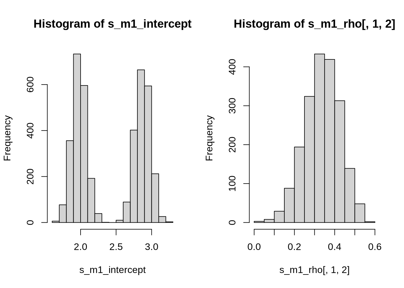
par(mfrow = c(1,1))
We see that the posterior of the intercepts are exactly what we expect. The same happens for the posterior of the correlation, which lies at around 0.35. Now, in principle, we can add any number of predictors to the previous model. Let us explore this.
First, we set some \(\beta\) parameter and x predictor. We will assume that \(\beta\) is shared across all outcomes in Y.
set.seed(1234)
x1 <- rnorm(100, 1.2, 0.5)
x2 <- rnorm(100, -2, 2)
beta <- 2.3
Y2 <- Y
Y2[,1] <- Y2[,1] + x1 * beta
Y2[,2] <- Y2[,2] + x2 * beta
And we can visualize what their joint distribution is now.
par(mfrow = c(1,2))
plot(Y[,1], Y[,2])
plot(Y2[,1], Y2[,2])
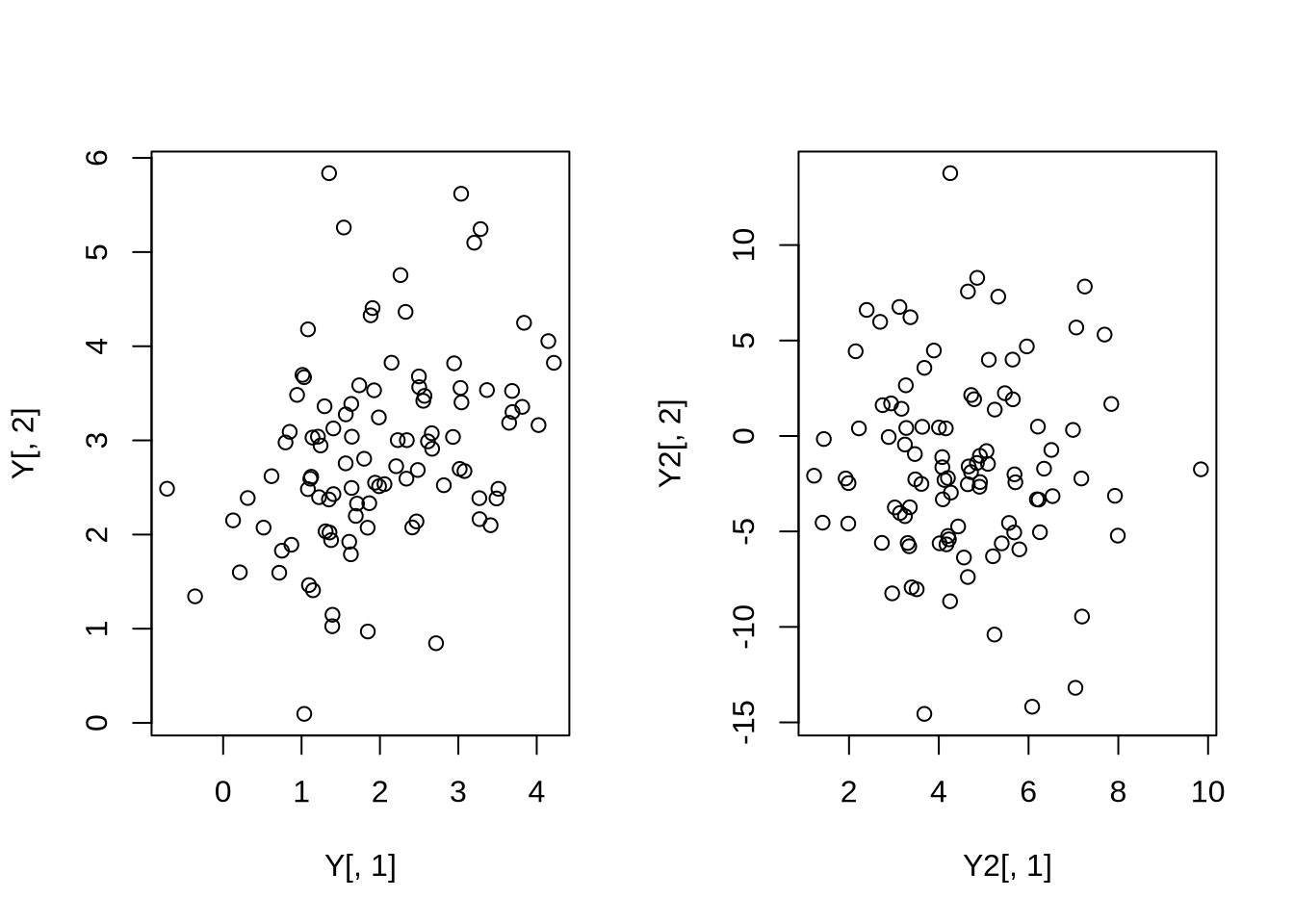
par(mfrow = c(1,1))
We see that the apparent correlation between the columns in Y is basically 0
round(cor(Y2), 2)
##       [,1]  [,2]
## [1,]  1.00 -0.03
## [2,] -0.03  1.00
What this means is that, given a confound, the real correlation between two variables can be heavily obscured. Let us try to model this like before, without taking into account the effect of the x1 and x2.
data_m2 <- list(
  N = 100
, K = 2
, Y = Y2
)

s2 <- sampling(m1
, data = data_m2
, iter = 1000
, warmup = 500
, cores = 4
, chains = 4
, seed = 1234)
And now we visualize the estimated correlation.
s_m2_rho <- rstan::extract(s2, "rho")$rho
hist(s_m2_rho[,1,2])
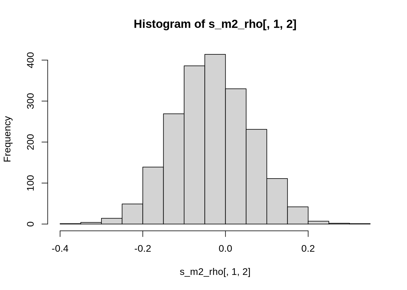
As expected, the estimated correlation coefficient rho is completely wrong. Let us try to build the correct model now.
model_2 <- "data {
  int N; // number of rows (observations)
  int K; // number of columns (variables)
  array[N] vector[K] Y;
  array[N] vector[K] X;
}
parameters {
  vector[K] intercept;  // intercepts
  real beta;            // beta estimate, recall we share beta across Yi
  corr_matrix[K] rho;   // correlation factor
  vector<lower=0>[K] sigma; // sigma
}
transformed parameters {
  matrix[N, K] mu;   // aggregated mean
  for(k in 1:K) {
    mu[,k] = intercept[k] + beta * to_vector(X[,k]);
  }
}
model {
  rho   ~ lkj_corr(2);       // generic prior on the correlation
  sigma ~ normal(0, 2);      // generic prior on sigma
  intercept  ~ normal(0, 2); // generic prior on intercept
  beta ~ normal(0, 2);       // generic prior on beta
  for (n in 1:N) {
    Y[n,] ~ multi_normal(mu[n,], quad_form_diag(rho, sigma));
  }
}"

m2 <- stan_model(model_code = model_2)

data_m3 <- list(
  N = 100
, K = 2
, Y = Y2
, X = cbind(x1, x2)
)

s3 <- sampling(m2
, data = data_m3
, iter = 1000
, warmup = 500
, cores = 4
, chains = 4
, seed = 1234)

print(s3, c("beta", "intercept", "rho"))
## Inference for Stan model: anon_model.
## 4 chains, each with iter=1000; warmup=500; thin=1;
## post-warmup draws per chain=500, total post-warmup draws=2000.
##
##              mean se_mean   sd 2.5%  25%  50%  75% 97.5% n_eff Rhat
## beta         2.37       0 0.05 2.28 2.34 2.37 2.40  2.46  1570    1
## intercept[1] 1.90       0 0.12 1.68 1.82 1.90 1.98  2.13  2120    1
## intercept[2] 3.01       0 0.14 2.73 2.91 3.01 3.10  3.28  1699    1
## rho[1,1]     1.00     NaN 0.00 1.00 1.00 1.00 1.00  1.00   NaN  NaN
## rho[1,2]     0.36       0 0.09 0.18 0.30 0.36 0.41  0.52  2286    1
## rho[2,1]     0.36       0 0.09 0.18 0.30 0.36 0.41  0.52  2286    1
## rho[2,2]     1.00       0 0.00 1.00 1.00 1.00 1.00  1.00  1803    1
##
## Samples were drawn using NUTS(diag_e) at Tue Jul 16 15:18:54 2024.
## For each parameter, n_eff is a crude measure of effective sample size,
## and Rhat is the potential scale reduction factor on split chains (at
## convergence, Rhat=1).
As you can see, now the estimates are spot on with what we expect. Before we move on to binary outcomes, let us take a look at what happens if we try to model Y as independent variables, without the correlation structure and parameter sharing.
model_3 <- "data {
  int N; // number of rows (observations)
  int K; // number of columns (variables)
  array[N] vector[K] Y;
  array[N] vector[K] X;
}
parameters {
  vector[K] intercept;  // intercepts
  vector[K] beta;       // beta estimate, but we do not share it
  vector<lower=0>[K] sigma; // sigma
}
transformed parameters {
  matrix[N, K] mu;   // aggregated mean
  for(k in 1:K) {
    mu[,k] = intercept[k] + beta[k] * to_vector(X[,k]);
  }
}
model {
  // the model is basically identical as before
  // but this time we model each Yi independently of each other
  sigma ~ normal(0, 2);      // generic prior on sigma
  intercept  ~ normal(0, 2); // generic prior on intercept
  beta ~ normal(0, 2);       // generic prior on beta
  for (k in 1:K) {
    Y[,k] ~ normal(mu[,k], sigma[k]);
  }
}"

m3 <- stan_model(model_code = model_3)

s4 <- sampling(m3
, data = data_m3
, iter = 1000
, warmup = 500
, cores = 4
, chains = 4
, seed = 1234)

print(s4, c("beta", "intercept"))
## Inference for Stan model: anon_model.
## 4 chains, each with iter=1000; warmup=500; thin=1;
## post-warmup draws per chain=500, total post-warmup draws=2000.
##
##              mean se_mean   sd 2.5%  25%  50%  75% 97.5% n_eff Rhat
## beta[1]      2.55    0.01 0.21 2.14 2.43 2.56 2.69  2.96  1328    1
## beta[2]      2.34    0.00 0.05 2.24 2.31 2.34 2.37  2.44  1421    1
## intercept[1] 1.69    0.01 0.25 1.19 1.52 1.69 1.87  2.18  1407    1
## intercept[2] 2.95    0.00 0.14 2.69 2.85 2.95 3.05  3.24  1442    1
##
## Samples were drawn using NUTS(diag_e) at Tue Jul 16 15:19:24 2024.
## For each parameter, n_eff is a crude measure of effective sample size,
## and Rhat is the potential scale reduction factor on split chains (at
## convergence, Rhat=1).
While the new results are close the estimates we got with the correct model, the new results are clearly further away from the real intercepts and beta coefficients.
Correlated binary outcomes
We can now finally move to binary outcomes. The principle is the same, we have multiple binary dependent variables which are correlated with eachother. There are multiple ways of generating correlated binary outcomes, but here is a simple one.
mu <- c(0.5, .2)
rho <- 0.7
Sigma <- diag(2) * (1 - rho) + rho
set.seed(1234)
Yb <- apply(rmvnorm(100, mean = mu, sigma = Sigma), 2, function(x) ifelse(x>=0, 1, 0))
head(Yb)
##      [,1] [,2]
## [1,]    0    1
## [2,]    1    0
## [3,]    1    1
## [4,]    0    0
## [5,]    0    0
## [6,]    0    0
We basically generate normally distributed correlated variables, and then convert them to binary by assuming that if Yi > 0, then it is 1, and 0 otherwise.
In principle, the stan model to capture correlated binary outcomes is very similar to the model to capture correlated normally distributed outcomes, but sadly there is no built in distribution to do this. However, we can define what is called a Multivariate Probit model. In this tutorial I will not explain how the core function of the MP model works, it should be taken as given.
This function works row by row. It takes a vector of dependent variables (y), a vector of means (mu), a special paramenter u, the number of of columns in y (K), and the lower cholesky decomposition of the correlation matrix (L_Omega).
model_4 <- "functions {
  real approx_Phi(real x) {
    return inv_logit(x * 1.702);
  }
  real approx_inv_Phi(real x) {
    return logit(x) / 1.702;
  }
  // this is our likelihood
  real multiprobit_lpmf(
    array[] int y,
    row_vector mu,    // Intercept
    array[] real u,
    int K,            // response dimension size
    matrix L_Omega    // lower cholesky of correlation matrix
  ){
    vector[K] z;       // latent continuous state
    vector[K] logLik;  // log likelihood
    real prev;
    prev = 0;
    for (k in 1:K) { // Phi and inv_Phi may overflow and / or be numerically inaccurate
      if (y[k] == -1 ) { // missing data gets ignored
        z[k] = L_Omega[k,k]*inv_Phi(u[k]);
    	logLik[k] = 0;
      }
      else {
        real bound; // threshold at which utility = 0
        bound = approx_Phi( -(mu[k] + prev) / L_Omega[k,k]  );
        if (y[k] == 1) {
          real t;
          t = bound + (1 - bound) * u[k];
          z[k] = approx_inv_Phi(t);       // implies utility is positive
          logLik[k] = log1m(bound);  // Jacobian adjustment
        }
        else {
          real t;
          t = bound * u[k];
          z[k] = approx_inv_Phi(t);       // implies utility is negative
          logLik[k]= log(bound);   // Jacobian adjustment
        }
      }
      if (k < K) prev = L_Omega[k+1,1:k] * head(z, k);
    }
    return sum(logLik);
  }
}
data {
  int N; // number of rows (observations)
  int K; // number of columns (variables)
  array[N, K] int <lower=-1, upper=1> Y;  // Actual outcomes
}
parameters {
  vector[K] intercept;  // intercepts
  cholesky_factor_corr[K] L_Omega;    // cholesky factor for correlation matrix for Y
  array[N,K] real<lower=0,upper=1> u; // special parameter
}
transformed parameters {
  // since we only have an intercept, we technically do not need this
  // but it is easier for the following models
  matrix[N, K] mu;
  for(k in 1:K) {
    mu[,k] = rep_vector(intercept[k], N);
  }
}
model {
  L_Omega    ~ lkj_corr_cholesky(2); // prior on correlation matrix
  intercept  ~ normal(0, 2);         // generic prior on intercept
  for(k in 1:K) {
    u[k] ~ beta(10,10);
  }
  for(n in 1:N) {
    target += multiprobit_lpmf(Y[n,] | mu[n,], u[n], K, L_Omega);
    // in this case we do not have the ~ statement
    // we need to use target += ...
  }
}
generated quantities {
  // since L_Omega is a choleschy decomposition
  // we need to build the cor matrix
  corr_matrix[K] Omega = multiply_lower_tri_self_transpose(L_Omega);
}"

m4 <- stan_model(model_code = model_4)

data_m4 <- list(
  N = 100
, K = 2
, Y = Yb
)

s5 <- sampling(m4
, data = data_m4
, iter = 1000
, warmup = 500
, cores = 4
, chains = 4
, seed = 1234)

print(s5, c("intercept", "Omega"))
## Inference for Stan model: anon_model.
## 4 chains, each with iter=1000; warmup=500; thin=1;
## post-warmup draws per chain=500, total post-warmup draws=2000.
##
##              mean se_mean   sd  2.5%   25%  50%  75% 97.5% n_eff Rhat
## intercept[1] 0.29       0 0.12  0.05  0.21 0.29 0.37  0.54  3279    1
## intercept[2] 0.08       0 0.13 -0.19 -0.01 0.07 0.16  0.33  3238    1
## Omega[1,1]   1.00     NaN 0.00  1.00  1.00 1.00 1.00  1.00   NaN  NaN
## Omega[1,2]   0.60       0 0.11  0.37  0.52 0.61 0.68  0.78  2372    1
## Omega[2,1]   0.60       0 0.11  0.37  0.52 0.61 0.68  0.78  2372    1
## Omega[2,2]   1.00       0 0.00  1.00  1.00 1.00 1.00  1.00  1541    1
##
## Samples were drawn using NUTS(diag_e) at Tue Jul 16 15:19:58 2024.
## For each parameter, n_eff is a crude measure of effective sample size,
## and Rhat is the potential scale reduction factor on split chains (at
## convergence, Rhat=1).
And that is basically it. We get an intercept and correlation matrix for the Yb. The same applies if we have predictors.
set.seed(1234)
x1 <- rnorm(100, 0.2, 0.5)
x2 <- rnorm(100, -0.5, 2)
beta <- 1.3

mu <- c(0.5, .2)
rho <- 0.7
Sigma <- diag(2) * (1 - rho) + rho
set.seed(1234)
Yb <- rmvnorm(100, mean = mu, sigma = Sigma)
Yb[,1] <- Yb[,1] + x1 * beta
Yb[,2] <- Yb[,2] + x2 * beta

Yb2 <- apply(Yb, 2, function(x) ifelse(x>=0, 1, 0))
Yb2
##        [,1] [,2]
##   [1,]    0    1
##   [2,]    1    0
##   [3,]    1    1
##   [4,]    0    0
##   [5,]    1    0
##   [6,]    1    0
##   [7,]    0    0
##   [8,]    1    1
##   [9,]    0    0
##  [10,]    1    1
##  [11,]    1    0
##  [12,]    0    0
##  [13,]    0    0
##  [14,]    1    1
##  [15,]    1    0
##  [16,]    1    1
##  [17,]    0    0
##  [18,]    0    0
##  [19,]    0    0
##  [20,]    1    0
##  [21,]    1    0
##  [22,]    0    0
##  [23,]    0    1
##  [24,]    0    0
##  [25,]    0    1
##  [26,]    0    0
##  [27,]    0    0
##  [28,]    1    0
##  [29,]    1    0
##  [30,]    1    0
##  [31,]    1    1
##  [32,]    1    0
##  [33,]    1    0
##  [34,]    0    1
##  [35,]    1    0
##  [36,]    0    0
##  [37,]    0    0
##  [38,]    1    0
##  [39,]    0    1
##  [40,]    1    0
##  [41,]    1    0
##  [42,]    0    1
##  [43,]    1    1
##  [44,]    1    0
##  [45,]    0    0
##  [46,]    1    1
##  [47,]    1    1
##  [48,]    0    1
##  [49,]    0    1
##  [50,]    1    1
##  [51,]    0    0
##  [52,]    1    0
##  [53,]    0    1
##  [54,]    0    0
##  [55,]    1    0
##  [56,]    1    1
##  [57,]    1    0
##  [58,]    1    0
##  [59,]    1    0
##  [60,]    1    0
##  [61,]    1    0
##  [62,]    1    1
##  [63,]    1    0
##  [64,]    0    0
##  [65,]    1    1
##  [66,]    1    1
##  [67,]    0    1
##  [68,]    0    0
##  [69,]    1    0
##  [70,]    1    1
##  [71,]    1    1
##  [72,]    1    0
##  [73,]    1    0
##  [74,]    1    0
##  [75,]    1    1
##  [76,]    1    0
##  [77,]    1    0
##  [78,]    1    1
##  [79,]    1    0
##  [80,]    0    0
##  [81,]    0    0
##  [82,]    1    0
##  [83,]    1    1
##  [84,]    1    1
##  [85,]    1    1
##  [86,]    1    1
##  [87,]    1    1
##  [88,]    1    0
##  [89,]    1    1
##  [90,]    1    0
##  [91,]    0    0
##  [92,]    1    0
##  [93,]    1    0
##  [94,]    1    1
##  [95,]    1    1
##  [96,]    0    0
##  [97,]    0    1
##  [98,]    1    0
##  [99,]    1    0
## [100,]    1    0
And then fit it.
model_5 <- "functions {
  real approx_Phi(real x) {
    return inv_logit(x * 1.702);
  }
  real approx_inv_Phi(real x) {
    return logit(x) / 1.702;
  }
  // this is our likelihood
  real multiprobit_lpmf(
			array[] int y,
			row_vector mu,    // Intercept
			array[] real u,
			int K,            // response dimension size
			matrix L_Omega    // lower cholesky of correlation matrix
			){
    vector[K] z;       // latent continuous state
    vector[K] logLik;  // log likelihood
    real prev;
    prev = 0;
    for (k in 1:K) { // Phi and inv_Phi may overflow and / or be numerically inaccurate
      if (y[k] == -1 ) { // missing data gets ignored
        z[k] = L_Omega[k,k]*inv_Phi(u[k]);
    	logLik[k] = 0;
      }
      else {
	    real bound; // threshold at which utility = 0
	    bound = approx_Phi( -(mu[k] + prev) / L_Omega[k,k]  );
	    if (y[k] == 1) {
	      real t;
	      t = bound + (1 - bound) * u[k];
	      z[k] = approx_inv_Phi(t);       // implies utility is positive
	      logLik[k] = log1m(bound);  // Jacobian adjustment
	    }
	    else {
	      real t;
	      t = bound * u[k];
	      z[k] = approx_inv_Phi(t);       // implies utility is negative
	      logLik[k]= log(bound);   // Jacobian adjustment
	    }
      }
      if (k < K) prev = L_Omega[k+1,1:k] * head(z, k);
    }
    return sum(logLik);
  }
}
data {
  int N; // number of rows (observations)
  int K; // number of columns (variables)
  array[N, K] int <lower=-1, upper=1> Y;  // Actual outcomes
  array[K] vector[N] X;
}
parameters {
  vector[K] intercept;  // intercepts
  cholesky_factor_corr[K] L_Omega;    // cholesky factor for correlation matrix for Y
  array[N,K] real<lower=0,upper=1> u; // special parameter
  real beta;
}
transformed parameters {
  // since we only have an intercept, we technically do not need this
  // but it is easier for the following models
  matrix[N, K] mu;
  for(k in 1:K) {
    mu[,k] = rep_vector(intercept[k], N) + beta * X[k];
  }
}
model {
  L_Omega    ~ lkj_corr_cholesky(2); // prior on correlation matrix
  intercept  ~ normal(0, 2);         // generic prior on intercept
  beta       ~ normal(0, 2);         // generic prior on beta
  for(k in 1:K) {
    u[k] ~ beta(10,10);
  }
  for(n in 1:N) {
    target += multiprobit_lpmf(Y[n,] | mu[n,], u[n], K, L_Omega);
    // in this case we do not have the ~ statement
    // we need to use target += ...
  }
}
generated quantities {
  // since L_Omega is a choleschy decomposition
  // we need to build the cor matrix
  corr_matrix[K] Omega = multiply_lower_tri_self_transpose(L_Omega);
}"

m5 <- stan_model(model_code = model_5)

data_m5 <- list(
  N = 100
, K = 2
, Y = Yb2
, X = rbind(x1, x2)
)

s6 <- sampling(m5
, data = data_m5
, iter = 1000
, warmup = 500
, cores = 4
, chains = 4
, seed = 1234)

print(s6, c("intercept", "Omega", "beta"))
## Inference for Stan model: anon_model.
## 4 chains, each with iter=1000; warmup=500; thin=1;
## post-warmup draws per chain=500, total post-warmup draws=2000.
##
##               mean se_mean   sd  2.5%   25%   50%   75% 97.5% n_eff Rhat
## intercept[1]  0.38    0.00 0.14  0.12  0.28  0.37  0.47  0.65  4504    1
## intercept[2] -0.23    0.00 0.19 -0.61 -0.36 -0.22 -0.09  0.16  2754    1
## Omega[1,1]    1.00     NaN 0.00  1.00  1.00  1.00  1.00  1.00   NaN  NaN
## Omega[1,2]    0.57    0.01 0.22  0.10  0.43  0.60  0.73  0.91  1345    1
## Omega[2,1]    0.57    0.01 0.22  0.10  0.43  0.60  0.73  0.91  1345    1
## Omega[2,2]    1.00    0.00 0.00  1.00  1.00  1.00  1.00  1.00  1886    1
## beta          1.53    0.00 0.26  1.06  1.35  1.53  1.70  2.07  3793    1
##
## Samples were drawn using NUTS(diag_e) at Tue Jul 16 15:20:35 2024.
## For each parameter, n_eff is a crude measure of effective sample size,
## and Rhat is the potential scale reduction factor on split chains (at
## convergence, Rhat=1).
As before, the estimates are rather close to the actual parameter values.
The final interesting aspect of this type of model is that we can do missing data inputation on the fly. Imagine we are missing some observations for some rows. We will code missing data as -1.
Yb3 <- Yb2
Yb3[6, 1] <- -1
Yb3[27, 2] <- -1
Yb3[56, 2] <- -1
Yb3[89, 1] <- -1
Now we can just run the exact same model but with the missing data.
data_m6 <- list(
  N = 100
, K = 2
, Y = Yb3
, X = rbind(x1, x2)
)

s7 <- sampling(m5
, data = data_m6
, iter = 1000
, warmup = 500
, cores = 4
, chains = 4
, seed = 1234)

print(s6, c("intercept", "Omega", "beta"))
## Inference for Stan model: anon_model.
## 4 chains, each with iter=1000; warmup=500; thin=1;
## post-warmup draws per chain=500, total post-warmup draws=2000.
##
##               mean se_mean   sd  2.5%   25%   50%   75% 97.5% n_eff Rhat
## intercept[1]  0.38    0.00 0.14  0.12  0.28  0.37  0.47  0.65  4504    1
## intercept[2] -0.23    0.00 0.19 -0.61 -0.36 -0.22 -0.09  0.16  2754    1
## Omega[1,1]    1.00     NaN 0.00  1.00  1.00  1.00  1.00  1.00   NaN  NaN
## Omega[1,2]    0.57    0.01 0.22  0.10  0.43  0.60  0.73  0.91  1345    1
## Omega[2,1]    0.57    0.01 0.22  0.10  0.43  0.60  0.73  0.91  1345    1
## Omega[2,2]    1.00    0.00 0.00  1.00  1.00  1.00  1.00  1.00  1886    1
## beta          1.53    0.00 0.26  1.06  1.35  1.53  1.70  2.07  3793    1
##
## Samples were drawn using NUTS(diag_e) at Tue Jul 16 15:20:35 2024.
## For each parameter, n_eff is a crude measure of effective sample size,
## and Rhat is the potential scale reduction factor on split chains (at
## convergence, Rhat=1).
print(s7, c("intercept", "Omega", "beta"))
## Inference for Stan model: anon_model.
## 4 chains, each with iter=1000; warmup=500; thin=1;
## post-warmup draws per chain=500, total post-warmup draws=2000.
##
##               mean se_mean   sd  2.5%   25%   50%   75% 97.5% n_eff Rhat
## intercept[1]  0.36    0.00 0.14  0.10  0.27  0.36  0.45  0.64  4600    1
## intercept[2] -0.23    0.00 0.20 -0.61 -0.36 -0.22 -0.09  0.16  3673    1
## Omega[1,1]    1.00     NaN 0.00  1.00  1.00  1.00  1.00  1.00   NaN  NaN
## Omega[1,2]    0.55    0.01 0.22  0.07  0.42  0.58  0.72  0.89  1302    1
## Omega[2,1]    0.55    0.01 0.22  0.07  0.42  0.58  0.72  0.89  1302    1
## Omega[2,2]    1.00    0.00 0.00  1.00  1.00  1.00  1.00  1.00  2074    1
## beta          1.51    0.00 0.25  1.06  1.33  1.49  1.67  2.05  3489    1
##
## Samples were drawn using NUTS(diag_e) at Tue Jul 16 15:20:40 2024.
## For each parameter, n_eff is a crude measure of effective sample size,
## and Rhat is the potential scale reduction factor on split chains (at
## convergence, Rhat=1).
The model runs as expected and the estimates are almost identical as with the full dataset. If we were interested in trying to recover the missing values they are in the model, in mu.
s7_mu <- colMeans(rstan::extract(s7, c("mu"))$mu)

data.frame(observed = c(Yb2[6, 1], Yb2[27, 2], Yb2[56, 2], Yb2[89, 1])
, imputation = as.integer(c(s7_mu[6, 1], s7_mu[27, 2], s7_mu[56, 2], s7_mu[89, 1])>0))
##   observed imputation
## 1        1          1
## 2        0          0
## 3        1          1
## 4        1          1
In this case, the model was able to perfectly recover all missing values. However, you should not expect that this is always the case, especially with linguistic data.
A case study: /p/ and /b/ in South America
We now have the tools to build a model looking at a realistic case study. For this case study we will look at a simple question: are two phonemes correlated, and if so, how strongly?. Let us start by getting the data.
phoibl <- read_csv("https://raw.githubusercontent.com/phoible/dev/master/data/phoible.csv")
## Rows: 105484 Columns: 49
## ── Column specification ─────────────────────────────────────────────────────────────────────────────────
## Delimiter: ","
## chr (47): Glottocode, ISO6393, LanguageName, SpecificDialect, GlyphID, Phone...
## dbl  (1): InventoryID
## lgl  (1): Marginal
##
## ℹ Use `spec()` to retrieve the full column specification for this data.
## ℹ Specify the column types or set `show_col_types = FALSE` to quiet this message.
glottolog <- read_csv("https://cdstar.eva.mpg.de//bitstreams/EAEA0-CFBC-1A89-0C8C-0/languages_and_dialects_geo.csv")
## Rows: 22111 Columns: 7
## ── Column specification ─────────────────────────────────────────────────────────────────────────────────
## Delimiter: ","
## chr (5): glottocode, name, isocodes, level, macroarea
## dbl (2): latitude, longitude
##
## ℹ Use `spec()` to retrieve the full column specification for this data.
## ℹ Specify the column types or set `show_col_types = FALSE` to quiet this message.
phoibl %>% head %>% as.data.frame()
##   InventoryID Glottocode ISO6393 LanguageName SpecificDialect   GlyphID Phoneme
## 1           1   kore1280     kor       Korean            <NA>      0068       h
## 2           1   kore1280     kor       Korean            <NA>      006A       j
## 3           1   kore1280     kor       Korean            <NA>      006B       k
## 4           1   kore1280     kor       Korean            <NA> 006B+02B0      kʰ
## 5           1   kore1280     kor       Korean            <NA> 006B+02C0      kˀ
## 6           1   kore1280     kor       Korean            <NA>      006C       l
##   Allophones Marginal SegmentClass Source tone stress syllabic short long
## 1      ç h ɦ       NA    consonant    spa    0      -        -     -    -
## 2          j       NA    consonant    spa    0      -        -     -    -
## 3      k̚ ɡ k       NA    consonant    spa    0      -        -     -    -
## 4         kʰ       NA    consonant    spa    0      -        -     -    -
## 5         kˀ       NA    consonant    spa    0      -        -     -    -
## 6     ɾ l lʲ       NA    consonant    spa    0      -        -     -    -
##   consonantal sonorant continuant delayedRelease approximant tap trill nasal
## 1           -        -          +              +           -   -     -     -
## 2           -        +          +              0           +   -     -     -
## 3           +        -          -              -           -   -     -     -
## 4           +        -          -              -           -   -     -     -
## 5           +        -          -              -           -   -     -     -
## 6           +        +          +              0           +   -     -     -
##   lateral labial round labiodental coronal anterior distributed strident dorsal
## 1       -      -     0           0       -        0           0        0      -
## 2       -      -     0           0       -        0           0        0      +
## 3       -      -     0           0       -        0           0        0      +
## 4       -      -     0           0       -        0           0        0      +
## 5       -      -     0           0       -        0           0        0      +
## 6       +      -     0           0       +        +           -        -      -
##   high low front back tense retractedTongueRoot advancedTongueRoot
## 1    0   0     0    0     0                   -                  -
## 2    +   -     +    -     +                   -                  -
## 3    +   -     -    -     0                   -                  -
## 4    +   -     -    -     0                   -                  -
## 5    +   -     -    -     0                   -                  -
## 6    0   0     0    0     0                   -                  -
##   periodicGlottalSource epilaryngealSource spreadGlottis constrictedGlottis
## 1                     -                  -             +                  -
## 2                     +                  -             -                  -
## 3                     -                  -             -                  -
## 4                     -                  -             +                  -
## 5                     -                  -             -                  +
## 6                     +                  -             -                  -
##   fortis lenis raisedLarynxEjective loweredLarynxImplosive click
## 1      -     -                    -                      -     -
## 2      -     -                    -                      -     -
## 3      -     -                    -                      -     -
## 4      -     -                    -                      -     -
## 5      -     -                    -                      -     -
## 6      -     -                    -                      -     -
glottolog %>% head %>% as.data.frame()
##   glottocode       name isocodes    level macroarea latitude longitude
## 1   3adt1234 3Ad-Tekles     <NA>  dialect    Africa       NA        NA
## 2   aala1237     Aalawa     <NA>  dialect Papunesia       NA        NA
## 3   aant1238 Aantantara     <NA>  dialect Papunesia       NA        NA
## 4   aari1239       Aari      aiw language    Africa  5.95034   36.5721
## 5   aari1240     Aariya      aay language   Eurasia       NA        NA
## 6   aasa1238      Aasax      aas language    Africa -4.00679   36.8648
Next, we filter only languages in South America.
langs_sa <- filter(glottolog, macroarea == "South America") %>% na.omit()
phoibl_sa <- filter(phoibl, Glottocode %in% langs_sa$glottocode)
phoibl_sa
## # A tibble: 12,272 × 49
##    InventoryID Glottocode ISO6393 LanguageName SpecificDialect GlyphID Phoneme
##          <dbl> <chr>      <chr>   <chr>        <chr>           <chr>   <chr>
##  1         101 chac1249   cbi     Cayapa       <NA>            0062    b
##  2         101 chac1249   cbi     Cayapa       <NA>            0063    c
##  3         101 chac1249   cbi     Cayapa       <NA>            0064    d
##  4         101 chac1249   cbi     Cayapa       <NA>            0068    h
##  5         101 chac1249   cbi     Cayapa       <NA>            006A    j
##  6         101 chac1249   cbi     Cayapa       <NA>            006B    k
##  7         101 chac1249   cbi     Cayapa       <NA>            006C    l
##  8         101 chac1249   cbi     Cayapa       <NA>            006D    m
##  9         101 chac1249   cbi     Cayapa       <NA>            006E    n
## 10         101 chac1249   cbi     Cayapa       <NA>            0070    p
## # ℹ 12,262 more rows
## # ℹ 42 more variables: Allophones <chr>, Marginal <lgl>, SegmentClass <chr>,
## #   Source <chr>, tone <chr>, stress <chr>, syllabic <chr>, short <chr>,
## #   long <chr>, consonantal <chr>, sonorant <chr>, continuant <chr>,
## #   delayedRelease <chr>, approximant <chr>, tap <chr>, trill <chr>,
## #   nasal <chr>, lateral <chr>, labial <chr>, round <chr>, labiodental <chr>,
## #   coronal <chr>, anterior <chr>, distributed <chr>, strident <chr>, …
Because phoibl includes multiple inventories for any single language, we choose one at random.
phoibl_sa_wide <- phoibl_sa %>% select(Glottocode, InventoryID, Phoneme) %>%
mutate(values = 1) %>%
pivot_wider(names_from = Phoneme, values_from = values, values_fill = 0)

set.seed(1234)
phoibl_sa_wide <- phoibl_sa_wide %>%
  group_by(Glottocode) %>%
  slice_sample(n = 1) %>%
  ungroup()

phoibl_sa_wide <- select(phoibl_sa_wide, Glottocode, b, p)
phoibl_sa_wide
## # A tibble: 330 × 3
##    Glottocode     b     p
##    <chr>      <dbl> <dbl>
##  1 abip1241       0     1
##  2 abis1238       0     1
##  3 acha1250       1     1
##  4 ache1246       1     1
##  5 achu1248       0     1
##  6 agua1253       0     1
##  7 aika1237       1     1
##  8 ajyi1238       0     1
##  9 akaw1239       1     1
## 10 akun1241       0     1
## # ℹ 320 more rows
The next step is to build a phylogenetic tree. There are many ways of doing this, but the easiest is to assume that the glottolog tree has the correct shape, and then assume that the branch lengths of the tree is proportional to the number of intermediate nodes in the tree. This assumption is not completely accurate, but it produces trees which are good enough for most modeling tasks.
We start by loading the glottolog tree in csv format (this is the languoid.csv files in glottolog)
languoid_url <- "https://cdstar.eva.mpg.de//bitstreams/EAEA0-CFBC-1A89-0C8C-0/glottolog_languoid.csv.zip"
download.file(url = languoid_url, destfile = "./languoid.csv.zip")
languoid <- read_csv("./languoid.csv.zip")
## Multiple files in zip: reading 'languoid.csv'
## Rows: 26879 Columns: 15
## ── Column specification ─────────────────────────────────────────────────────────────────────────────────
## Delimiter: ","
## chr (7): id, family_id, parent_id, name, level, iso639P3code, country_ids
## dbl (5): latitude, longitude, child_family_count, child_language_count, chil...
## lgl (3): bookkeeping, description, markup_description
##
## ℹ Use `spec()` to retrieve the full column specification for this data.
## ℹ Specify the column types or set `show_col_types = FALSE` to quiet this message.
languoid
## # A tibble: 26,879 × 15
##    id       family_id parent_id name       bookkeeping level  latitude longitude
##    <chr>    <chr>     <chr>     <chr>      <lgl>       <chr>     <dbl>     <dbl>
##  1 3adt1234 afro1255  nort3292  3Ad-Tekles FALSE       diale…    NA         NA
##  2 aala1237 aust1307  ramo1244  Aalawa     FALSE       diale…    NA         NA
##  3 aant1238 nucl1709  nort2920  Aantantara FALSE       diale…    NA         NA
##  4 aari1238 sout2845  ahkk1235  Aari-Gayil FALSE       family    NA         NA
##  5 aari1239 sout2845  aari1238  Aari       FALSE       langu…     5.95      36.6
##  6 aari1240 book1242  book1242  Aariya     TRUE        langu…    NA         NA
##  7 aasa1238 afro1255  sout3054  Aasax      FALSE       langu…    -4.01      36.9
##  8 aasd1234 indo1319  ferr1240  Aasdring   FALSE       diale…    NA         NA
##  9 aata1238 nucl1709  sout2943  Aatasaara  FALSE       diale…    NA         NA
## 10 abaa1238 sino1245  nort3305  Rngaba     FALSE       diale…    NA         NA
## # ℹ 26,869 more rows
## # ℹ 7 more variables: iso639P3code <chr>, description <lgl>,
## #   markup_description <lgl>, child_family_count <dbl>,
## #   child_language_count <dbl>, child_dialect_count <dbl>, country_ids <chr>
Next, we define some functions to travel through the glottolog tree.
## this is the main function to traverse the chain
get_chain <- function(.id, db) {
    cid <- .id
    pid <- get_parent(cid, db)
    chain <- c(.id, pid)
    while(!is.na(pid)) {
        pid <- get_parent(cid, db)
        if(!is.na(pid))
            chain <- c(chain, pid)
        cid <- pid
    }
    chain <- chain[!is.na(chain)]
    return(chain)
}
get_names <- function(.idf, db = families)
    sapply(.idf, function(.id)
        db[db$id == .id, ]$name)
get_parent <- function(.id, db = families){
    db[db$id == .id, ]$parent_id
}
build_phylos <- function(.lfd, .var, db, .micro_family = FALSE
                      , distance = FALSE) {
    .var <- enquo(.var)
    ## extract family chain
    chains <- sapply(.lfd$id,
                    function(x) {
                      c(get_names(get_chain(x, db), db), "TOP__")
                    })
    ## get the family chains
    chain.1 <- chains %>% sapply(function(x)(paste(x, collapse = ";")))
    if(.micro_family)
        chain.1 <- sapply(chain.1, function(x) str_remove(x, "^.*?;"))
    all.vals <- unique(unlist(strsplit(chain.1, ";")))
    all.vals <- all.vals[!is.na(all.vals)]
    ## build dataframes
    df.philo <- select(.lfd, !!.var)
    for(col in all.vals){
      df.philo[,col] <- as.integer(str_detect(chain.1, col))
    }
    df.philo <- distinct(df.philo)
    df.philo_d <- dist.b(df.philo)
    if (distance) {
        df.philo_d
    } else {
        as.dist(1/df.philo_d) %>%
            hclust() %>%
            as.phylo()
    }
}
## distance function
dist.b <- function(X) {
    m <- as.matrix(as.data.frame(X)[,-1])
    rownames(m) <- as.data.frame(X)[,1]
    m <- cbind(1:nrow(m), m)
    apply(m, 1, function(r) {
        cat(r[1], "/", nrow(m), "- ", sep="")
        r[r==0] <- -1
        rowSums(t(t(m[,-1])==r[-1]))
    })
}
And then build a dataframe with all the information:
## build family dataset
## extract language data
lang_gloto_data <- languoid %>%
    select(id, family_id, parent_id, name)
fam_ids <- languoid %>% pull(family_id)
fam_gloto_data <- languoid %>%
    select(id, name)
## we do a double left join to have the data in two columns
lang_fam_gloto_data <-
    left_join(lang_gloto_data,
              fam_gloto_data,
              by = c("family_id" = "id"),
              suffix = c("_language", "_macro_family")) %>%
    left_join(fam_gloto_data,
              by = c("parent_id" = "id"),
              suffix = c("_macro_family", "_micro_family")) %>%
    rename(name_micro_family = name) %>%
    mutate(name_micro_family =
               case_when(is.na(name_micro_family) ~ name_language,
                         TRUE ~ name_micro_family),
           name_macro_family =
               case_when(is.na(name_macro_family) ~ name_language,
                         TRUE ~ name_macro_family))
## this contains the tree in the format we need it
Finally, we build the distances to get the actual branch lenghts. The correlation structure of the tree is in df_phylo_cor.
lfd <- filter(lang_fam_gloto_data, id %in% phoibl_sa_wide$Glottocode)
df_phylo <- build_phylos(lfd, id, db = languoid, .micro_family = FALSE)
## 1/330- 2/330- 3/330- 4/330- 5/330- 6/330- 7/330- 8/330- 9/330- 10/330- 11/330- 12/330- 13/330- 14/330- 15/330- 16/330- 17/330- 18/330- 19/330- 20/330- 21/330- 22/330- 23/330- 24/330- 25/330- 26/330- 27/330- 28/330- 29/330- 30/330- 31/330- 32/330- 33/330- 34/330- 35/330- 36/330- 37/330- 38/330- 39/330- 40/330- 41/330- 42/330- 43/330- 44/330- 45/330- 46/330- 47/330- 48/330- 49/330- 50/330- 51/330- 52/330- 53/330- 54/330- 55/330- 56/330- 57/330- 58/330- 59/330- 60/330- 61/330- 62/330- 63/330- 64/330- 65/330- 66/330- 67/330- 68/330- 69/330- 70/330- 71/330- 72/330- 73/330- 74/330- 75/330- 76/330- 77/330- 78/330- 79/330- 80/330- 81/330- 82/330- 83/330- 84/330- 85/330- 86/330- 87/330- 88/330- 89/330- 90/330- 91/330- 92/330- 93/330- 94/330- 95/330- 96/330- 97/330- 98/330- 99/330- 100/330- 101/330- 102/330- 103/330- 104/330- 105/330- 106/330- 107/330- 108/330- 109/330- 110/330- 111/330- 112/330- 113/330- 114/330- 115/330- 116/330- 117/330- 118/330- 119/330- 120/330- 121/330- 122/330- 123/330- 124/330- 125/330- 126/330- 127/330- 128/330- 129/330- 130/330- 131/330- 132/330- 133/330- 134/330- 135/330- 136/330- 137/330- 138/330- 139/330- 140/330- 141/330- 142/330- 143/330- 144/330- 145/330- 146/330- 147/330- 148/330- 149/330- 150/330- 151/330- 152/330- 153/330- 154/330- 155/330- 156/330- 157/330- 158/330- 159/330- 160/330- 161/330- 162/330- 163/330- 164/330- 165/330- 166/330- 167/330- 168/330- 169/330- 170/330- 171/330- 172/330- 173/330- 174/330- 175/330- 176/330- 177/330- 178/330- 179/330- 180/330- 181/330- 182/330- 183/330- 184/330- 185/330- 186/330- 187/330- 188/330- 189/330- 190/330- 191/330- 192/330- 193/330- 194/330- 195/330- 196/330- 197/330- 198/330- 199/330- 200/330- 201/330- 202/330- 203/330- 204/330- 205/330- 206/330- 207/330- 208/330- 209/330- 210/330- 211/330- 212/330- 213/330- 214/330- 215/330- 216/330- 217/330- 218/330- 219/330- 220/330- 221/330- 222/330- 223/330- 224/330- 225/330- 226/330- 227/330- 228/330- 229/330- 230/330- 231/330- 232/330- 233/330- 234/330- 235/330- 236/330- 237/330- 238/330- 239/330- 240/330- 241/330- 242/330- 243/330- 244/330- 245/330- 246/330- 247/330- 248/330- 249/330- 250/330- 251/330- 252/330- 253/330- 254/330- 255/330- 256/330- 257/330- 258/330- 259/330- 260/330- 261/330- 262/330- 263/330- 264/330- 265/330- 266/330- 267/330- 268/330- 269/330- 270/330- 271/330- 272/330- 273/330- 274/330- 275/330- 276/330- 277/330- 278/330- 279/330- 280/330- 281/330- 282/330- 283/330- 284/330- 285/330- 286/330- 287/330- 288/330- 289/330- 290/330- 291/330- 292/330- 293/330- 294/330- 295/330- 296/330- 297/330- 298/330- 299/330- 300/330- 301/330- 302/330- 303/330- 304/330- 305/330- 306/330- 307/330- 308/330- 309/330- 310/330- 311/330- 312/330- 313/330- 314/330- 315/330- 316/330- 317/330- 318/330- 319/330- 320/330- 321/330- 322/330- 323/330- 324/330- 325/330- 326/330- 327/330- 328/330- 329/330- 330/330-
df_phylo_cor <- ape::vcv.phylo(df_phylo, corr = TRUE)
Next, we need to build some distances for the spatial component. While we could try to go with different types of distance metrics like topographic distances, these can be hard to compute. In this example I will use geodesic distances.
phoibl_sa_wide <- left_join(phoibl_sa_wide, select(glottolog, glottocode, latitude, longitude)
, by = c("Glottocode" = "glottocode"))
dist_mat <- geodist(select(phoibl_sa_wide, latitude, longitude), measure = "geodesic")/100000
round(dist_mat[1:5, 1:5], 2)
##       [,1]  [,2]  [,3]  [,4]  [,5]
## [1,]  0.00 34.12 38.84  5.87 33.70
## [2,] 34.12  0.00  7.04 33.50  2.96
## [3,] 38.84  7.04  0.00 37.26  9.76
## [4,]  5.87 33.50 37.26  0.00 33.61
## [5,] 33.70  2.96  9.76 33.61  0.00
Notice we divide the distance matrix by 1000000. This is technically not strictly necessary, but as explained in the post on Gaussian Processes, it is easier to sample for parameters on smaller numbers. With these elements we can now build the model.
model_mv_code <- "
functions{
  // this is our Kernel, other kernelts are possible
  matrix cov_matern52(matrix D, real sdgp, real lscale) {
    int N = dims(D)[1];
    matrix[N, N] K;
    for (i in 1:(N - 1)) {
      K[i, i] = sdgp^2;
      for (j in (i + 1):N) {
	real x52 = (sqrt(5) * D[i,j])/lscale;
	K[i, j] = sdgp^2 *
	  (1 + x52 + (x52^2)/3)* exp(-x52);
	K[j, i] = K[i, j];
      }
    }
    K[N, N] = sdgp^2;
    return K;
  }
  real approx_Phi(real x) {
    return inv_logit(x * 1.702);
  }
  real approx_inv_Phi(real x) {
    return logit(x) / 1.702;
  }
  real multiprobit_lpmf(
    array[] int y,
    row_vector mu,    // Intercept
    array[] real u,
    int K,            // response dimension size
    matrix L_Omega    // lower cholesky of correlation matrix
  ){
    vector[K] z;       // latent continuous state
    vector[K] logLik;  // log likelihood
    real prev;
    prev = 0;
    for (k in 1:K) { // Phi and inv_Phi may overflow and / or be numerically inaccurate
      if (y[k] == -1 ) { // missing data gets ignored
        z[k] = L_Omega[k,k]*inv_Phi(u[k]);
    	logLik[k] = 0;
      }
      else {
        real bound; // threshold at which utility = 0
        bound = approx_Phi( -(mu[k] + prev) / L_Omega[k,k]  );
        if (y[k] == 1) {
          real t;
          t = bound + (1 - bound) * u[k];
          z[k] = approx_inv_Phi(t);       // implies utility is positive
          logLik[k] = log1m(bound);  // Jacobian adjustment
        }
        else {
          real t;
          t = bound * u[k];
          z[k] = approx_inv_Phi(t);       // implies utility is negative
          logLik[k]= log(bound);   // Jacobian adjustment
        }
      }
      if (k < K) prev = L_Omega[k+1,1:k] * head(z, k);
    }
    return sum(logLik);
  }
}
data {
  int<lower=0>                    N;         // Sample size
  int<lower=0>                    K;         // Number of outcomes (2 in our case)
  matrix[N,  N]                   dist_mat;  // spatial distances
  array [N, K] int<lower=-1, upper=1> Y;         // dependent variables
  matrix[N , N]                   cov_phylo; // phylogenetic correlation
}
parameters {
  cholesky_factor_corr[K] L_Omega;   // cholesky factor for correlation matrix for Y
  real<lower=0,upper=1>   u[N,K];   // nuisance that absorbs inequality constraints
  // linear part
  array[K] real          intercept;
  // gp stuff
  array[K] vector[N]     zgp;       // latent part
  real<lower=0>          lscale;    // length scale
  real<lower=0>          sdgp;      // sd of the GP
  // phylogenetic
  array[K] vector[N]     eta_phylo; // group effects
  array[K] real<lower=0> eta_sd;    // sd of group effects
}
transformed parameters {
  matrix[N, K] mu;
  matrix[N, N] LCov;
  {
    // notice we 'share' lscale and sdgp across outcomes
    matrix[N, N] Kov = cov_matern52(dist_mat, sdgp, lscale);
    LCov = cholesky_decompose(add_diag(Kov, 1e-10));
    for (k in 1:K) {
      mu[, k] = intercept[k] + LCov * zgp[k] + eta_sd[k] * (cov_phylo * eta_phylo[k]);
    }
  }
}
model {
  // intercepts + linear
  L_Omega   ~ lkj_corr_cholesky(4); // tighter prior on L_Omega
  intercept ~ normal(0, 2);    // generic prior on the intercept
  lscale    ~ inv_gamma(4, 2); // this parameter is hard to get right
  sdgp      ~ normal(0, 2);    // generic prior on sd gp
  eta_sd    ~ normal(0, 2);
  for(k in 1:K) {
    u[k]         ~ beta(10, 10);
    zgp[k]       ~ std_normal();
    eta_phylo[k] ~ std_normal();
  }
  { // likelihood for neighbors
    for(n in 1:N){
      target += multiprobit_lpmf(Y[n] | mu[n], u[n], K, L_Omega);
    }
  }
}
generated quantities {
  corr_matrix[K] Omega = multiply_lower_tri_self_transpose(L_Omega);
}"
model_mv <- stan_model(model_code = model_mv_code)
Because this takes a loooong time to fit, we take a smaller sample from the data first.
set.seed(1234)
samples <- sample(1:nrow(phoibl_sa_wide), 100)
samples
##   [1] 284 101 111 133  98 103 214  90  79 270 184  62   4 149  40 212 195  93
##  [19] 122  66 175 304 108 131  41 115 228 298 299 258 117 322 182 320 221 224
##  [37]  49 136 282 145 123 264 234  96  22 208 307  57  10 248 153 330  83 245
##  [55] 281 218 215 169  71  61 155  60  36  19 137 126 158 116 291 102 324  85
##  [73] 259 160  77  17 194 265   6 186 130 181 285  11 269 100 163 275 309  21
##  [91] 170 261 134   9 171 267 286 174 316  29
phoibl_sa_wide_s <- phoibl_sa_wide[samples, ]
phoibl_sa_wide_s
## # A tibble: 100 × 5
##    Glottocode     b     p latitude longitude
##    <chr>      <dbl> <dbl>    <dbl>     <dbl>
##  1 urub1250       0     1    -2.46     -46.2
##  2 guaj1255       0     1    -4.69     -45.7
##  3 hual1241       0     1    -9.57     -75.6
##  4 kain1272       1     1   -27.8      -52.5
##  5 gali1262       1     1     5.84     -56.8
##  6 guam1248       0     1     2.56     -76.6
##  7 para1311       0     1   -25.6      -57.1
##  8 embe1260       1     0     7.53     -76.7
##  9 cube1242       1     1     1.32     -70.2
## 10 ticu1245       1     1    -3.66     -69.9
## # ℹ 90 more rows
data_mv <- list(
K = 2
, N = nrow(phoibl_sa_wide_s)
, Y = select(phoibl_sa_wide_s, p, b)
, dist_mat = dist_mat[samples, samples]
, cov_phylo = t(chol(df_phylo_cor[samples, samples])) ## we need the choleschy factor, but R does it the wrong way round
)

s_mv <- sampling(model_mv
, data = data_mv
, iter = 1000
, warmup = 500
, chains = 4
, cores  = 4
, seed   = 1234)
## Warning: Bulk Effective Samples Size (ESS) is too low, indicating posterior means and medians may be unreliable.
## Running the chains for more iterations may help. See
## https://mc-stan.org/misc/warnings.html#bulk-ess
The model samples well, but it complains about low ESS. In this case we do not care because this is just for illustration purposes. We can explore the posterior samples.
print(s_mv, c("intercept", "Omega"))
## Inference for Stan model: anon_model.
## 4 chains, each with iter=1000; warmup=500; thin=1;
## post-warmup draws per chain=500, total post-warmup draws=2000.
##
##               mean se_mean   sd  2.5%   25%   50%   75% 97.5% n_eff Rhat
## intercept[1]  2.51    0.04 0.86  1.30  1.86  2.36  3.01  4.62   454 1.01
## intercept[2] -0.33    0.02 0.43 -1.29 -0.55 -0.31 -0.08  0.48   664 1.01
## Omega[1,1]    1.00     NaN 0.00  1.00  1.00  1.00  1.00  1.00   NaN  NaN
## Omega[1,2]   -0.26    0.01 0.29 -0.76 -0.46 -0.28 -0.07  0.38   624 1.01
## Omega[2,1]   -0.26    0.01 0.29 -0.76 -0.46 -0.28 -0.07  0.38   624 1.01
## Omega[2,2]    1.00    0.00 0.00  1.00  1.00  1.00  1.00  1.00  1489 1.00
##
## Samples were drawn using NUTS(diag_e) at Tue Jul 16 15:22:29 2024.
## For each parameter, n_eff is a crude measure of effective sample size,
## and Rhat is the potential scale reduction factor on split chains (at
## convergence, Rhat=1).
We get a perhaps unexpected result, namely that /p/ and /b/ are negatively correlated in this small dataset. The lscale and sdgp parameters are as follows
print(s_mv, c("lscale", "sdgp"))
## Inference for Stan model: anon_model.
## 4 chains, each with iter=1000; warmup=500; thin=1;
## post-warmup draws per chain=500, total post-warmup draws=2000.
##
##        mean se_mean   sd 2.5%  25%  50%  75% 97.5% n_eff Rhat
## lscale 0.71    0.02 0.45 0.23 0.41 0.61 0.88  1.77   716 1.00
## sdgp   1.01    0.05 0.74 0.04 0.41 0.86 1.46  2.69   220 1.01
##
## Samples were drawn using NUTS(diag_e) at Tue Jul 16 15:22:29 2024.
## For each parameter, n_eff is a crude measure of effective sample size,
## and Rhat is the potential scale reduction factor on split chains (at
## convergence, Rhat=1).
Now, the final thing we can look at is the spatial structures the model found. Building spatial conditional effects with multivariate probit models is somewhat more complex than with regular logistic or probit models, and it can be very slow because we have to sample from a multivariate normal distribution.
The first step is to define some functions for the covariance kernel. Here, cov_mat52 calculates the matern52 covariance given a distance matrix, the lscale and sdgp parameters.
cov_mat52 <- function(d, lscale, sdgp) {
  m52 <- (sqrt(5)*d)/lscale
  sdgp^2 * (1 + m52 + (m52^2)/3)* exp(-m52)
}
Next, we need to define a function for the predictive distribution of a Gaussian Process. It is given below. This function takes the new cross distance matrix, yL is the zgp parameter in the model, cov_fun the covariance function, pars the parameters for the covariance function (lscale and sdgp), L_Sigma is the Cholesky decomposition of the covariance function applied to the old distance with the estimated parameters (LCov in the model).
This function is technically missing a portion of the structure, since it only generates the mean of the posterior. I have commented out the missing code. In my experience, there is effectively no difference between using the mean of the posterior (mu_yL_new) and sampling from the multivariate normal including the uncertainty and correlation in cov_yL_new. It has also been my experience that this step usually fails for numerical reasons unless you use Euclidean distances. Finally, because new_dist is the square matrix of new distances, you need to split your predictions into manageable chunks (say 100 new observations), otherwise it takes forever.
predictor_gp <- function(new_dist_cross
                       , yL
                       , cov_fun
                       , lscale
                       , sdgp
                       , L_Sigma
                       ## , new_dist
) {
  L_Sigma_inverse <- solve(L_Sigma)
  K_div_yL <- L_Sigma_inverse %*% yL
  K_div_yL <- t(t(K_div_yL) %*% L_Sigma_inverse)
  k_x_x_new <- t(cov_fun(d = new_dist_cross, lscale = lscale, sdgp = sdgp))
  mu_yL_new <- as.numeric(t(k_x_x_new) %*% K_div_yL)
  mu_yL_new
  ## lx_new <- nrow(new_dist)
  ## v_new <- L_Sigma_inverse %*% k_x_x_new
  ## cov_yL_new <- cov_fun(dd = new_dist, pars = pars) -
    ## t(v_new) %*% v_new + diag(rep(nug, lx_new), lx_new, lx_new)
  ## yL_new <- rmvnorm(1, mean = mu_yL_new, sigma = cov_yL_new)
  ## yL_new
}
Finally, we need a function to make the actual predictions from the model. This function will vary according to actual structure of the model, of course, but here is a basic template. old_dist is the distance matrix of the observations used to fit the model, new_dist is the crossed distance from new observations to old, cov_fun the covariance function, n_samples how many samples to use for the predictions, sample the actual model samples, mc.cores to make predictions in parallel.
predict_model <- function(new_dist
                        , cov_fun
                        , n_samples
                        , samples
                        , mc.cores = 1) {
  pars <- rstan::extract(samples)
  s_lscale <- pars$lscale
  s_sdgp <- pars$sdgp
  s_intercept <- pars$intercept
  s_zgp <- pars$zgp
  s_omega <- pars$Omega
  s_GP_mat <- pars$LCov
  ## make prediction matrix
  K <- ncol(s_intercept)
  N <- nrow(new_dist)
  mu <- matrix(NA, ncol = K, nrow = N) ## we will make the predictions here
  n_samples2 <- sample(1:nrow(s_lscale), n_samples)
  mclapply (n_samples2, function(j) {
    message(j)
    for (k in 1:K) {
      if (length(dim(s_sdgp)) == 2) {
        ## no parameter sharing (not our case, but we include it)
        s_sdgp_jk <- s_sdgp[j,k]
        s_lscale_jk <- s_lscale[j,k]
      } else if(length(dim(s_sdgp)) == 1) {
        ## if there is only one lscale and sdgp
        s_sdgp_jk <- s_sdgp[j]
        s_lscale_jk <- s_lscale[j]
      }
      ## make LCov
      mu[,k] <- s_intercept[j,k] +
        predictor_gp(
          new_dist_cross = new_dist,
          yL = s_GP_mat[j,,] %*% s_zgp[j,k,],
          cov_fun = cov_fun,
          sdgp = s_sdgp_jk,
          lscale = s_lscale_jk,
          L_Sigma = s_GP_mat[j,,]
        )
    }
    preds <- matrix(NA, ncol = K, nrow = N)
    for(n in 1:(N)) {
      preds[n,] <- as.integer(rmvnorm(n=1
                                    , mean = as.vector(mu[n,])
                                    , sigma = s_omega[j,,])>0)
    }
    preds
  }, mc.cores = mc.cores)
}
Finally, to be able to build the spatial structure, we need to create a gird of points for which we want to make predictions. To do this, we define a rectangle containing all observations in our data, and set a grid filling that rectangle.
max_lat <- max(phoibl_sa_wide_s$latitude) + 1
min_lat <- min(phoibl_sa_wide_s$latitude) - 1
max_lon <- max(phoibl_sa_wide_s$longitude) + 1
min_lon <- min(phoibl_sa_wide_s$longitude) - 1

seq_lon <- seq(from = min_lon, to = max_lon, by = 0.4)
seq_lat <- seq(from = min_lat, to = max_lat, by = 0.4)

new_data <- tibble(
lon = rep(seq_lon, length(seq_lat))
, lat = rep(seq_lat, each = length(seq_lon)))
new_data
## # A tibble: 13,617 × 2
##      lon   lat
##    <dbl> <dbl>
##  1 -80.2 -48.6
##  2 -79.8 -48.6
##  3 -79.4 -48.6
##  4 -79.0 -48.6
##  5 -78.6 -48.6
##  6 -78.2 -48.6
##  7 -77.8 -48.6
##  8 -77.4 -48.6
##  9 -77.0 -48.6
## 10 -76.6 -48.6
## # ℹ 13,607 more rows
We then need to calculate the distance from each location (row) in new_data to each location in the data used to fit the model
dist_new_cross <- geodist::geodist(new_data, select(phoibl_sa_wide_s, longitude, latitude)
, measure = "geodesic")
dist_new_cross <- dist_new_cross/100000
new_dist_mat <- geodist(new_data, measure = "geodesic")
And make the predictions
set.seed(1234)
spatial_preds_mp <- predict_model(
  dist_new_cross
, cov_fun = cov_mat52
, n_samples = 100
, samples = s_mv
, mc.cores = 1)

write_rds(spatial_preds_mp, "./spatial-preds.rds")
With the predictions, we can now make a map. First we need to take the mean of the posterior predictions.
mean_sp_preds <- (Reduce("+", spatial_preds_mp)/100) %>%
cbind(new_data) %>%
as_tibble() %>%
rename(phoneme_p = `1`, phoneme_b = `2`)
And then we can just plot it. In theory, we could also add some map shp to the plot, but I will keep it simple for this tutorial.
Sys.setenv(PROJ_DATA = "/home/matias/miniforge3/envs/env-phylogenetic-blog/share/proj")

sa_shp <- ne_countries(continent = "South America")

ggplot() +
  geom_tile(data = mean_sp_preds, aes(x = lon, y = lat, fill = phoneme_b))+
  geom_point(data = phoibl_sa_wide_s, aes(x = longitude, y = latitude, shape = as.factor(b))
  , color = "#E84646") +
  geom_sf(data = sa_shp, fill = NA, color = "black")
## Warning: The `scale_name` argument of `continuous_scale()` is deprecated as of ggplot2 3.5.0.
## This warning is displayed once every 8 hours.
## Call `lifecycle::last_lifecycle_warnings()` to see where this warning was generated.
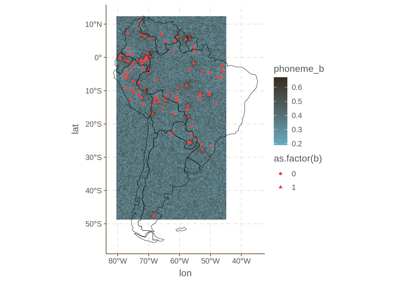
Which does seem to track, to an extent, the areas without /b/. Next we can look at /p/:
ggplot() +
  geom_tile(data = mean_sp_preds, aes(x = lon, y = lat, fill = phoneme_p))+
  geom_point(data = phoibl_sa_wide_s, aes(x = longitude, y = latitude, shape = as.factor(p))
  , color = "#E84646") +
  geom_sf(data = sa_shp, fill = NA, color = "black")
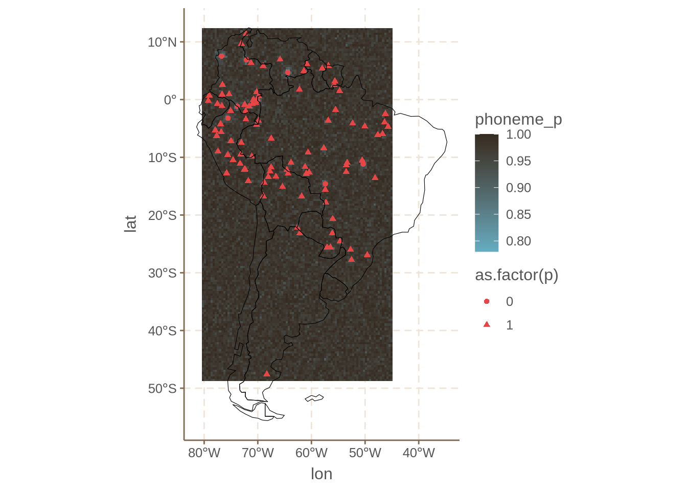
Which shows a much weaker pattern. This corresponds well to the fact most languages do have /p/ in the dataset. It also shows that feature choice matters. In general, it is ideal to choose phonemes which show some degree of variationa (that is, not too common or too uncommon).
Conclusion
In this post I have introduced the main idea of multivAreate. MultivAreate allows us to model multiple binary dependent variables, with potentially missing data, simulataneously and as correlated. It also allows us to share parameters across multiple dependent variables. This is an extremely flexible model for spatial and typological questions.