This entry is on the concept, implementation and optimization of phylogenetic regression terms. If you find this tutorial useful, pleace cite the following paper.
Guzmán Naranjo, Matías and Becker, Laura. “Statistical bias control in typology” Linguistic Typology, vol. 26, no. 3, 2022, pp. 605-670. https://doi.org/10.1515/lingty-2021-0002
Phylogenetic regression terms
When we model linguistic features the most prominent confound is that languages are related to each other and thus, observations are not independent from each other. The most common way to “control” for genetic confound is to add the language family as an effect to the model. Often this is done with so-called “random-“effects, which simply means effects with shrinkage. We will call these group-level effects.
We start loading the necessary libraries.
library(tidyverse)
## ── Attaching core tidyverse packages ───────────────────────────────────────────────── tidyverse 2.0.0 ──
## ✔ dplyr     1.1.4     ✔ readr     2.1.5
## ✔ forcats   1.0.0     ✔ stringr   1.5.1
## ✔ ggplot2   3.5.1     ✔ tibble    3.2.1
## ✔ lubridate 1.9.3     ✔ tidyr     1.3.1
## ✔ purrr     1.0.2
## ── Conflicts ─────────────────────────────────────────────────────────────────── tidyverse_conflicts() ──
## ✖ dplyr::filter() masks stats::filter()
## ✖ dplyr::lag()    masks stats::lag()
## ℹ Use the conflicted package (<http://conflicted.r-lib.org/>) to force all conflicts to become errors
library(geodist)
library(rnaturalearth)
library(rstan)
## Loading required package: StanHeaders
##
## rstan version 2.32.6 (Stan version 2.32.2)
##
## For execution on a local, multicore CPU with excess RAM we recommend calling
## options(mc.cores = parallel::detectCores()).
## To avoid recompilation of unchanged Stan programs, we recommend calling
## rstan_options(auto_write = TRUE)
## For within-chain threading using `reduce_sum()` or `map_rect()` Stan functions,
## change `threads_per_chain` option:
## rstan_options(threads_per_chain = 1)
##
##
## Attaching package: 'rstan'
##
## The following object is masked from 'package:tidyr':
##
##     extract
library(tidybayes)
library(brms)
## Loading required package: Rcpp
## Loading 'brms' package (version 2.20.1). Useful instructions
## can be found by typing help('brms'). A more detailed introduction
## to the package is available through vignette('brms_overview').
##
## Attaching package: 'brms'
##
## The following objects are masked from 'package:tidybayes':
##
##     dstudent_t, pstudent_t, qstudent_t, rstudent_t
##
## The following object is masked from 'package:rstan':
##
##     loo
##
## The following object is masked from 'package:stats':
##
##     ar
library(sf)
## Linking to GEOS 3.12.2, GDAL 3.9.1, PROJ 9.4.1; sf_use_s2() is TRUE
library(ape)
##
## Attaching package: 'ape'
##
## The following object is masked from 'package:dplyr':
##
##     where
## devtools::install_github('Mikata-Project/ggthemr')
library(ggthemr)
ggthemr("fresh")

## you probably don't need this
setwd("~/Documentos/Uni/blog/content/post/2024-07-04-phylogenetic-regression/")
Sys.setenv(PROJ_DATA = "/home/matias/miniforge3/envs/env-phylogenetic-blog/share/proj")
Concept
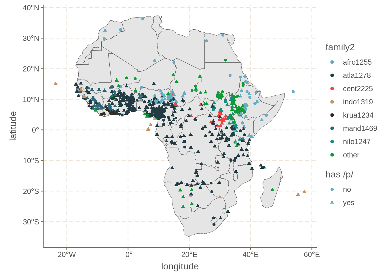
We will start by visualizing how the problem originates. Here is the data we will use for this case study. The question we want to answer is rather simple: other things being equal, what is the probability of /p/ in a language in Africa?
phoibl <- read_csv("https://raw.githubusercontent.com/phoible/dev/master/data/phoible.csv")
## Rows: 105484 Columns: 49
## ── Column specification ─────────────────────────────────────────────────────────────────────────────────
## Delimiter: ","
## chr (47): Glottocode, ISO6393, LanguageName, SpecificDialect, GlyphID, Phone...
## dbl  (1): InventoryID
## lgl  (1): Marginal
##
## ℹ Use `spec()` to retrieve the full column specification for this data.
## ℹ Specify the column types or set `show_col_types = FALSE` to quiet this message.
glottolog <- read_csv("https://cdstar.eva.mpg.de//bitstreams/EAEA0-CFBC-1A89-0C8C-0/languages_and_dialects_geo.csv")
## Rows: 22111 Columns: 7
## ── Column specification ─────────────────────────────────────────────────────────────────────────────────
## Delimiter: ","
## chr (5): glottocode, name, isocodes, level, macroarea
## dbl (2): latitude, longitude
##
## ℹ Use `spec()` to retrieve the full column specification for this data.
## ℹ Specify the column types or set `show_col_types = FALSE` to quiet this message.
afr_glotto <- filter(glottolog, macroarea == "Africa") %>% pull(glottocode)

phoibl_afr <- filter(phoibl, Glottocode %in% afr_glotto)

set.seed(1234)
phoibl_afr_wide <- select(phoibl_afr, InventoryID, Glottocode, Phoneme) %>%
  mutate(value = 1) %>%
  pivot_wider(names_from = Phoneme, values_from = value, values_fill = 0) %>%
  group_by(Glottocode) %>%
  slice_sample(n = 1) %>%
  ungroup() %>%
  select(Glottocode, p)

languoid_url <- "https://cdstar.eva.mpg.de//bitstreams/EAEA0-CFBC-1A89-0C8C-0/glottolog_languoid.csv.zip"
download.file(url = languoid_url, destfile = "./languoid.csv.zip")
languoid <- read_csv("./languoid.csv.zip")
## Multiple files in zip: reading 'languoid.csv'
## Rows: 26879 Columns: 15
## ── Column specification ─────────────────────────────────────────────────────────────────────────────────
## Delimiter: ","
## chr (7): id, family_id, parent_id, name, level, iso639P3code, country_ids
## dbl (5): latitude, longitude, child_family_count, child_language_count, chil...
## lgl (3): bookkeeping, description, markup_description
##
## ℹ Use `spec()` to retrieve the full column specification for this data.
## ℹ Specify the column types or set `show_col_types = FALSE` to quiet this message.
phoibl_afr_wide <-
  left_join(phoibl_afr_wide, select(languoid, id, family_id, longitude, latitude),
    by = c("Glottocode" = "id")
  )
fams <- table(phoibl_afr_wide$family_id)

phoibl_afr_wide$family2 <-
  ifelse(phoibl_afr_wide$family_id %in% names(fams[fams > 10]), phoibl_afr_wide$family_id, "other")
The family bias issue should be visible in the following map.
africa_shp <- ne_countries(continent = "Africa")
ggplot() +
  geom_sf(data = africa_shp) +
  geom_point(
    data = phoibl_afr_wide,
    aes(
      x = longitude, y = latitude, color = family2,
      shape = as.factor(ifelse(p==1, "yes", "no"))
    )
  ) +
  scale_shape(name = "has /p/")
## Warning: The `scale_name` argument of `discrete_scale()` is deprecated as of ggplot2 3.5.0.
## This warning is displayed once every 8 hours.
## Call `lifecycle::last_lifecycle_warnings()` to see where this warning was generated.
## Warning: Removed 23 rows containing missing values or values outside the scale
## range (`geom_point()`).
Also, we can calculate the within-family proportion of /p/.
p_family <- table(phoibl_afr_wide$family_id)
## only families with more than 10 members
families_2 <- names(p_family[p_family>10])
phoibl_afr_wide_s <- filter(phoibl_afr_wide, family_id %in% families_2)
table(phoibl_afr_wide_s$p, phoibl_afr_wide_s$family_id)
##
##     afro1255 atla1278 cent2225 indo1319 krua1234 mand1469 nilo1247
##   0       32       63        0        0        0        4        3
##   1       68      348       23       11       11       39       24
round(prop.table(table(phoibl_afr_wide_s$p, phoibl_afr_wide_s$family_id), 2), 2)
##
##     afro1255 atla1278 cent2225 indo1319 krua1234 mand1469 nilo1247
##   0     0.32     0.15     0.00     0.00     0.00     0.09     0.11
##   1     0.68     0.85     1.00     1.00     1.00     0.91     0.89
As you can see, some falies like Afro-Asiatic (afro1255) have considerably more 0s than families like Mande (mand1469). This strongly suggests that there is a genetic bias in how common /p/ is in these languages.
Group-effects on family
Before moving to phylogenetic regression we will take a look at what happens without any type of controls and then we will use the traditional approach: one coefficient per family. The idea is that whatever bias there is in the data, it can be summarized at the family level (sometimes people will use Genus instead of family, but the idea is the same).
First to a model without any controls.
model_1 <- "
data {
  int N;
  array[N] int y;
}
parameters {
  real intercept;
}
transformed parameters {
  vector[N] mu;
  mu = rep_vector(intercept, N);
}
model {
  intercept ~ normal(0, 2);
  y ~ bernoulli_logit(mu);
}
"
m1 <- stan_model(model_code = model_1)
The previous model is pretty standard: we assume y is distributed as a bernoulli variable, with probability equal to the intercept (in logit scale, and we do not have any predictors). We can fit the model as follows.
data_1 <- list(
  N = nrow(phoibl_afr_wide)
, y = phoibl_afr_wide$p
)
s1 <- sampling(m1, data = data_1, iter = 1000, warmup = 500, seed = 1234, cores = 4, chains = 4)
print(s1, "intercept")
## Inference for Stan model: anon_model.
## 4 chains, each with iter=1000; warmup=500; thin=1;
## post-warmup draws per chain=500, total post-warmup draws=2000.
##
##           mean se_mean   sd 2.5%  25%  50%  75% 97.5% n_eff Rhat
## intercept 1.54       0 0.09 1.37 1.48 1.54 1.61  1.73   739    1
##
## Samples were drawn using NUTS(diag_e) at Tue Jul 16 15:24:29 2024.
## For each parameter, n_eff is a crude measure of effective sample size,
## and Rhat is the potential scale reduction factor on split chains (at
## convergence, Rhat=1).
This model works as expected with an intercept of 1.54. Since this paramenter is in logit scale, we need to transform it to get a real probability.
round(brms::inv_logit_scaled(1.54), 2)
## [1] 0.82
Which gives us 0.82, which happens to be basically the proportion of /p/ in our data.
round(sum(phoibl_afr_wide$p)/nrow(phoibl_afr_wide), 2)
## [1] 0.82
Basically, the model tells us that the probability of /p/, all other things being equal, is 0.82. This is rather uninformative because we know that family bias plays a real role in the distribution of linguistic features in the world’s languages. The first idea is to include family as a predictor. We will use shrinkage to estimate the effect of family.
model_2 <- "
data {
  int N;
  int N_fam;
  array[N] int y;
  array[N] int family_id;
}
parameters {
  real intercept;
  vector[N_fam] family_eff_centered;
  real i_family;
  real<lower=0> sd_family;
}
transformed parameters {
  vector[N] mu;
  vector[N_fam] family_eff = family_eff_centered * sd_family + i_family;
  for (n in 1:N) {
      mu[n] = intercept + family_eff[family_id[n]];
  }
}
model {
  intercept ~ normal(0, 2);
  i_family  ~ normal(0, 2);
  sd_family ~ exponential(1);
  family_eff_centered ~ std_normal(); // recall the non-centered parametrization
  y ~ bernoulli_logit(mu);
}
"
m2 <- stan_model(model_code = model_2)
And we can sample as follows.
phoibl_afr_wide$family_id2 <- ifelse(is.na(phoibl_afr_wide$family_id),
  "other", phoibl_afr_wide$family_id
) %>% as.factor()

data_2 <- list(
  N = nrow(phoibl_afr_wide),
  N_fam = length(unique(phoibl_afr_wide$family_id2)),
  y = phoibl_afr_wide$p,
  family_id = as.integer(phoibl_afr_wide$family_id2)
)

s2 <- sampling(m2, data = data_2, iter = 1000, warmup = 500, seed = 1243, cores = 4)
print(s2, c("intercept", "i_family", "sd_family"))
## Inference for Stan model: anon_model.
## 4 chains, each with iter=1000; warmup=500; thin=1;
## post-warmup draws per chain=500, total post-warmup draws=2000.
##
##           mean se_mean   sd  2.5%   25%  50%  75% 97.5% n_eff Rhat
## intercept 0.86    0.04 1.42 -1.90 -0.08 0.85 1.84  3.67  1163    1
## i_family  0.87    0.04 1.42 -1.90 -0.08 0.87 1.82  3.67  1162    1
## sd_family 1.30    0.02 0.47  0.55  0.96 1.26 1.56  2.42   608    1
##
## Samples were drawn using NUTS(diag_e) at Tue Jul 16 15:25:02 2024.
## For each parameter, n_eff is a crude measure of effective sample size,
## and Rhat is the potential scale reduction factor on split chains (at
## convergence, Rhat=1).
round(brms::inv_logit_scaled(0.86), 2)
## [1] 0.7
We see that the intercept moved quite a bit to 0.85, which in probability scale is 0.7. Meaning that the effect of family clearly biases the result of the model without any sort of family controls.
We can also visualize what happens to each family.
family_eff <- extract(s2, "family_eff")$family_eff

family_eff_df <-
  family_eff %>%
  as.data.frame() %>%
  as_tibble() %>%
  set_names(levels(phoibl_afr_wide$family_id2)) %>%
  mutate(sample = 1:n()) %>%
  pivot_longer(-sample)

ggplot() +
  stat_histinterval(data = family_eff_df, aes(y = name, x = value))
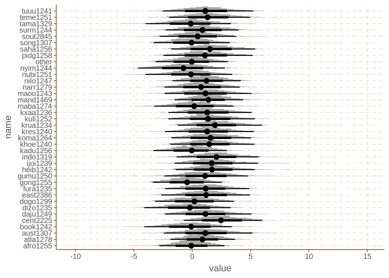
We see the effect of family is relatively weak if we go by the posteriors, with maybe the exception of Sudanic (cent2225). Nonetheless, the impact on the intercept is very noticeable. This is often a pattern with these types of models: the fact that we get “weak” or “non-significant” (in frequentist terms) effects, has little bearing on whether we should keep those predictors or not. What matters is whether the effects make sense for the model or not.
The problem with the previous model is that it assumes that all languages within each family behave the same. It does not take into account the fact that two languages which are close in a family tree, will be more similar than two languages in very different branches. For example, we would expect Spanish and Catalan to be more similar than Spanish and Farsi.
Slow implementation
The idea of phylogenetic regression is that we want to include the information of the whole tree into our model. We want to be able to distinguish between closely related languages and less closely related languages. The first step towards this is to get a language tree. We will use glottolog.
There are different ways of accessing the glottolog tree, here I will present an example with the languoid.csv file (already loaded). This file has one languoid (dialect, language or family) per row. It also contains information about the top level family (family_id) and the immediate parent of the languoid (parent_id). What this means is that we can get a whole tree branch by traversing from child to parent.
languoid
## # A tibble: 26,879 × 15
##    id       family_id parent_id name       bookkeeping level  latitude longitude
##    <chr>    <chr>     <chr>     <chr>      <lgl>       <chr>     <dbl>     <dbl>
##  1 3adt1234 afro1255  nort3292  3Ad-Tekles FALSE       diale…    NA         NA
##  2 aala1237 aust1307  ramo1244  Aalawa     FALSE       diale…    NA         NA
##  3 aant1238 nucl1709  nort2920  Aantantara FALSE       diale…    NA         NA
##  4 aari1238 sout2845  ahkk1235  Aari-Gayil FALSE       family    NA         NA
##  5 aari1239 sout2845  aari1238  Aari       FALSE       langu…     5.95      36.6
##  6 aari1240 book1242  book1242  Aariya     TRUE        langu…    NA         NA
##  7 aasa1238 afro1255  sout3054  Aasax      FALSE       langu…    -4.01      36.9
##  8 aasd1234 indo1319  ferr1240  Aasdring   FALSE       diale…    NA         NA
##  9 aata1238 nucl1709  sout2943  Aatasaara  FALSE       diale…    NA         NA
## 10 abaa1238 sino1245  nort3305  Rngaba     FALSE       diale…    NA         NA
## # ℹ 26,869 more rows
## # ℹ 7 more variables: iso639P3code <chr>, description <lgl>,
## #   markup_description <lgl>, child_family_count <dbl>,
## #   child_language_count <dbl>, child_dialect_count <dbl>, country_ids <chr>
The following functions are used to build the tree. The function dist.b is a distance function to get the distance between any two tips of the tree. This distance assumes that branch length is proportional to number of shared nodes in the tree. Technically, this is a simplification because branch length will depend on how detailed the tree is. However, this is in my experience more than good enough. There are some alternatives to try and get more realistic branch lengths, but I am unware of any realistic advantage.
get_chain <- function(.id, db) {
  cid <- .id
  pid <- get_parent(cid, db)
  chain <- c(.id, pid)
  while(!is.na(pid)) {
    pid <- get_parent(cid, db)
    if(!is.na(pid))
      chain <- c(chain, pid)
    cid <- pid
  }
  chain <- chain[!is.na(chain)]
  return(chain)
}
get_names <- function(.idf, db = families)
  sapply(.idf, function(.id)
    db[db$id == .id, ]$name)
get_parent <- function(.id, db = families){
  db[db$id == .id, ]$parent_id
}
build_phylos <- function(.lfd, .var, db, .micro_family = FALSE
                       , distance = FALSE) {
  .var <- enquo(.var)
  ## extract family chain
  chains <- sapply(.lfd$id,
    function(x) {
      c(get_names(get_chain(x, db), db), "TOP__")
    })
  ## get the family chains
  chain.1 <- chains %>% sapply(function(x)(paste(x, collapse = ";")))
  if(.micro_family)
    chain.1 <- sapply(chain.1, function(x) str_remove(x, "^.*?;"))
  all.vals <- unique(unlist(strsplit(chain.1, ";")))
  all.vals <- all.vals[!is.na(all.vals)]
  ## build dataframes
  df.philo <- select(.lfd, !!.var)
  for(col in all.vals){
    df.philo[,col] <- as.integer(str_detect(chain.1, col))
  }
  df.philo <- distinct(df.philo)
  df.philo_d <- dist.b(df.philo)
  if (distance) {
    df.philo_d
  } else {
    as.dist(1/df.philo_d) %>%
      hclust() %>%
      as.phylo()
  }
}
## distance function
dist.b <- function(X) {
  m <- as.matrix(as.data.frame(X)[,-1])
  rownames(m) <- as.data.frame(X)[,1]
  m <- cbind(1:nrow(m), m)
  apply(m, 1, function(r) {
    cat(r[1], "/", nrow(m), "- ", sep="")
    r[r==0] <- -1
    rowSums(t(t(m[,-1])==r[-1]))
  })
}
The next step is to build the data and calculate the distance
## build family dataset
## extract language data
lang_gloto_data <- languoid %>%
    select(id, family_id, parent_id, name)
fam_ids <- languoid %>% pull(family_id)
fam_gloto_data <- languoid %>%
    select(id, name)
## we do a double left join to have the data in two columns
lang_fam_gloto_data <-
    left_join(lang_gloto_data,
              fam_gloto_data,
              by = c("family_id" = "id"),
              suffix = c("_language", "_macro_family")) %>%
    left_join(fam_gloto_data,
              by = c("parent_id" = "id"),
              suffix = c("_macro_family", "_micro_family")) %>%
    rename(name_micro_family = name) %>%
    mutate(name_micro_family =
               case_when(is.na(name_micro_family) ~ name_language,
                         TRUE ~ name_micro_family),
           name_macro_family =
               case_when(is.na(name_macro_family) ~ name_language,
                         TRUE ~ name_macro_family))
## this contains the tree in the format we need it
And we build the tree and calculate the phylogenetic correlation from the distance. This is done with the ape::vcv.phylo function
lfd <- filter(lang_fam_gloto_data, id %in% phoibl_afr_wide$Glottocode)
df_phylo <- build_phylos(lfd, id, db = languoid, .micro_family = FALSE)
## 1/718- 2/718- 3/718- 4/718- 5/718- 6/718- 7/718- 8/718- 9/718- 10/718- 11/718- 12/718- 13/718- 14/718- 15/718- 16/718- 17/718- 18/718- 19/718- 20/718- 21/718- 22/718- 23/718- 24/718- 25/718- 26/718- 27/718- 28/718- 29/718- 30/718- 31/718- 32/718- 33/718- 34/718- 35/718- 36/718- 37/718- 38/718- 39/718- 40/718- 41/718- 42/718- 43/718- 44/718- 45/718- 46/718- 47/718- 48/718- 49/718- 50/718- 51/718- 52/718- 53/718- 54/718- 55/718- 56/718- 57/718- 58/718- 59/718- 60/718- 61/718- 62/718- 63/718- 64/718- 65/718- 66/718- 67/718- 68/718- 69/718- 70/718- 71/718- 72/718- 73/718- 74/718- 75/718- 76/718- 77/718- 78/718- 79/718- 80/718- 81/718- 82/718- 83/718- 84/718- 85/718- 86/718- 87/718- 88/718- 89/718- 90/718- 91/718- 92/718- 93/718- 94/718- 95/718- 96/718- 97/718- 98/718- 99/718- 100/718- 101/718- 102/718- 103/718- 104/718- 105/718- 106/718- 107/718- 108/718- 109/718- 110/718- 111/718- 112/718- 113/718- 114/718- 115/718- 116/718- 117/718- 118/718- 119/718- 120/718- 121/718- 122/718- 123/718- 124/718- 125/718- 126/718- 127/718- 128/718- 129/718- 130/718- 131/718- 132/718- 133/718- 134/718- 135/718- 136/718- 137/718- 138/718- 139/718- 140/718- 141/718- 142/718- 143/718- 144/718- 145/718- 146/718- 147/718- 148/718- 149/718- 150/718- 151/718- 152/718- 153/718- 154/718- 155/718- 156/718- 157/718- 158/718- 159/718- 160/718- 161/718- 162/718- 163/718- 164/718- 165/718- 166/718- 167/718- 168/718- 169/718- 170/718- 171/718- 172/718- 173/718- 174/718- 175/718- 176/718- 177/718- 178/718- 179/718- 180/718- 181/718- 182/718- 183/718- 184/718- 185/718- 186/718- 187/718- 188/718- 189/718- 190/718- 191/718- 192/718- 193/718- 194/718- 195/718- 196/718- 197/718- 198/718- 199/718- 200/718- 201/718- 202/718- 203/718- 204/718- 205/718- 206/718- 207/718- 208/718- 209/718- 210/718- 211/718- 212/718- 213/718- 214/718- 215/718- 216/718- 217/718- 218/718- 219/718- 220/718- 221/718- 222/718- 223/718- 224/718- 225/718- 226/718- 227/718- 228/718- 229/718- 230/718- 231/718- 232/718- 233/718- 234/718- 235/718- 236/718- 237/718- 238/718- 239/718- 240/718- 241/718- 242/718- 243/718- 244/718- 245/718- 246/718- 247/718- 248/718- 249/718- 250/718- 251/718- 252/718- 253/718- 254/718- 255/718- 256/718- 257/718- 258/718- 259/718- 260/718- 261/718- 262/718- 263/718- 264/718- 265/718- 266/718- 267/718- 268/718- 269/718- 270/718- 271/718- 272/718- 273/718- 274/718- 275/718- 276/718- 277/718- 278/718- 279/718- 280/718- 281/718- 282/718- 283/718- 284/718- 285/718- 286/718- 287/718- 288/718- 289/718- 290/718- 291/718- 292/718- 293/718- 294/718- 295/718- 296/718- 297/718- 298/718- 299/718- 300/718- 301/718- 302/718- 303/718- 304/718- 305/718- 306/718- 307/718- 308/718- 309/718- 310/718- 311/718- 312/718- 313/718- 314/718- 315/718- 316/718- 317/718- 318/718- 319/718- 320/718- 321/718- 322/718- 323/718- 324/718- 325/718- 326/718- 327/718- 328/718- 329/718- 330/718- 331/718- 332/718- 333/718- 334/718- 335/718- 336/718- 337/718- 338/718- 339/718- 340/718- 341/718- 342/718- 343/718- 344/718- 345/718- 346/718- 347/718- 348/718- 349/718- 350/718- 351/718- 352/718- 353/718- 354/718- 355/718- 356/718- 357/718- 358/718- 359/718- 360/718- 361/718- 362/718- 363/718- 364/718- 365/718- 366/718- 367/718- 368/718- 369/718- 370/718- 371/718- 372/718- 373/718- 374/718- 375/718- 376/718- 377/718- 378/718- 379/718- 380/718- 381/718- 382/718- 383/718- 384/718- 385/718- 386/718- 387/718- 388/718- 389/718- 390/718- 391/718- 392/718- 393/718- 394/718- 395/718- 396/718- 397/718- 398/718- 399/718- 400/718- 401/718- 402/718- 403/718- 404/718- 405/718- 406/718- 407/718- 408/718- 409/718- 410/718- 411/718- 412/718- 413/718- 414/718- 415/718- 416/718- 417/718- 418/718- 419/718- 420/718- 421/718- 422/718- 423/718- 424/718- 425/718- 426/718- 427/718- 428/718- 429/718- 430/718- 431/718- 432/718- 433/718- 434/718- 435/718- 436/718- 437/718- 438/718- 439/718- 440/718- 441/718- 442/718- 443/718- 444/718- 445/718- 446/718- 447/718- 448/718- 449/718- 450/718- 451/718- 452/718- 453/718- 454/718- 455/718- 456/718- 457/718- 458/718- 459/718- 460/718- 461/718- 462/718- 463/718- 464/718- 465/718- 466/718- 467/718- 468/718- 469/718- 470/718- 471/718- 472/718- 473/718- 474/718- 475/718- 476/718- 477/718- 478/718- 479/718- 480/718- 481/718- 482/718- 483/718- 484/718- 485/718- 486/718- 487/718- 488/718- 489/718- 490/718- 491/718- 492/718- 493/718- 494/718- 495/718- 496/718- 497/718- 498/718- 499/718- 500/718- 501/718- 502/718- 503/718- 504/718- 505/718- 506/718- 507/718- 508/718- 509/718- 510/718- 511/718- 512/718- 513/718- 514/718- 515/718- 516/718- 517/718- 518/718- 519/718- 520/718- 521/718- 522/718- 523/718- 524/718- 525/718- 526/718- 527/718- 528/718- 529/718- 530/718- 531/718- 532/718- 533/718- 534/718- 535/718- 536/718- 537/718- 538/718- 539/718- 540/718- 541/718- 542/718- 543/718- 544/718- 545/718- 546/718- 547/718- 548/718- 549/718- 550/718- 551/718- 552/718- 553/718- 554/718- 555/718- 556/718- 557/718- 558/718- 559/718- 560/718- 561/718- 562/718- 563/718- 564/718- 565/718- 566/718- 567/718- 568/718- 569/718- 570/718- 571/718- 572/718- 573/718- 574/718- 575/718- 576/718- 577/718- 578/718- 579/718- 580/718- 581/718- 582/718- 583/718- 584/718- 585/718- 586/718- 587/718- 588/718- 589/718- 590/718- 591/718- 592/718- 593/718- 594/718- 595/718- 596/718- 597/718- 598/718- 599/718- 600/718- 601/718- 602/718- 603/718- 604/718- 605/718- 606/718- 607/718- 608/718- 609/718- 610/718- 611/718- 612/718- 613/718- 614/718- 615/718- 616/718- 617/718- 618/718- 619/718- 620/718- 621/718- 622/718- 623/718- 624/718- 625/718- 626/718- 627/718- 628/718- 629/718- 630/718- 631/718- 632/718- 633/718- 634/718- 635/718- 636/718- 637/718- 638/718- 639/718- 640/718- 641/718- 642/718- 643/718- 644/718- 645/718- 646/718- 647/718- 648/718- 649/718- 650/718- 651/718- 652/718- 653/718- 654/718- 655/718- 656/718- 657/718- 658/718- 659/718- 660/718- 661/718- 662/718- 663/718- 664/718- 665/718- 666/718- 667/718- 668/718- 669/718- 670/718- 671/718- 672/718- 673/718- 674/718- 675/718- 676/718- 677/718- 678/718- 679/718- 680/718- 681/718- 682/718- 683/718- 684/718- 685/718- 686/718- 687/718- 688/718- 689/718- 690/718- 691/718- 692/718- 693/718- 694/718- 695/718- 696/718- 697/718- 698/718- 699/718- 700/718- 701/718- 702/718- 703/718- 704/718- 705/718- 706/718- 707/718- 708/718- 709/718- 710/718- 711/718- 712/718- 713/718- 714/718- 715/718- 716/718- 717/718- 718/718-
df_phylo_cor <- ape::vcv.phylo(df_phylo, corr = TRUE)
The phylogenetic correlation matrix looks as follows.
round(df_phylo_cor[1:5, 1:5], 2)
##          aari1239 abar1238 abid1235 abua1244 abur1243
## aari1239        1     0.00     0.00     0.00     0.00
## abar1238        0     1.00     0.67     0.75     0.67
## abid1235        0     0.67     1.00     0.67     0.80
## abua1244        0     0.75     0.67     1.00     0.67
## abur1243        0     0.67     0.80     0.67     1.00
With this matrix in place, the next step is to build the model. The idea is that we went to have a coefficient per language instead of one coefficient per family. However, we also want to enforce that the coefficients respect the structure of the tree. We do this by sampling from a multivariate normal distribution, with Sigma proportional to the correlation matrix above. Recall the MultivariateNormal(mu, Sigma) is equal to CSigma * Normal(0, 1) + mu, where the CSigma is the cholesky factor of Sigma.
model_3 <- "
data {
  int N;
  array[N] int y;
  array[N] int phylo_id; // now this indicates the glottocode index for each lang
  matrix[N,N] phylo_chol_corr;
}
parameters {
  real intercept;
  vector[N] phylo_eff_centered;  // N length because we have one per language
  real<lower=0> sd_phylo;
}
transformed parameters {
  vector[N] mu;
  vector[N] phylo_eff = (phylo_chol_corr * phylo_eff_centered) * sd_phylo;
  for (n in 1:N) {
      mu[n] = intercept + phylo_eff[phylo_id[n]];
  }
}
model {
  intercept ~ normal(0, 2);
  sd_phylo ~ exponential(4);
  phylo_eff_centered ~ std_normal(); // recall the non-centered parametrization
  y ~ bernoulli_logit(mu);
}
"
m3 <- stan_model(model_code = model_3)
And we can sample the model as follows.
data_3 <- list(
  N = nrow(phoibl_afr_wide),
  y = phoibl_afr_wide$p,
  phylo_id = as.integer(as.factor(phoibl_afr_wide$Glottocode)),
  phylo_chol_corr = t(chol(df_phylo_cor))
)

s3 <- sampling(m3, data = data_3, iter = 1000, warmup = 500, seed = 1234, cores = 4)
## Warning: Bulk Effective Samples Size (ESS) is too low, indicating posterior means and medians may be unreliable.
## Running the chains for more iterations may help. See
## https://mc-stan.org/misc/warnings.html#bulk-ess
print(s3, c("intercept", "sd_phylo"))
## Inference for Stan model: anon_model.
## 4 chains, each with iter=1000; warmup=500; thin=1;
## post-warmup draws per chain=500, total post-warmup draws=2000.
##
##           mean se_mean   sd 2.5%  25%  50%  75% 97.5% n_eff Rhat
## intercept 2.10    0.02 0.47 1.27 1.76 2.07 2.41  3.07   744 1.00
## sd_phylo  2.36    0.03 0.49 1.55 2.01 2.31 2.66  3.43   314 1.01
##
## Samples were drawn using NUTS(diag_e) at Tue Jul 16 15:25:54 2024.
## For each parameter, n_eff is a crude measure of effective sample size,
## and Rhat is the potential scale reduction factor on split chains (at
## convergence, Rhat=1).
The results are quite different from the model with only family effects, but I will discuss them bellow.
Fast implementation
Now, while the previous model works as expected, it is not as efficient as it could be. The reason is that we are wasting a for loop. The line with mu[n] = intercept + phylo_eff[phylo_id[n]]; is unnecesary because phylo_id is just 1:nrow(phoibl_afr_wide), that is, a sequence of integers from 1 to N. But this is the same as simply adding intercept + phylo_eff; in one go. Let us try that.
model_4 <- "
data {
  int N;
  array[N] int y;
  matrix[N,N] phylo_chol_corr;
}
parameters {
  real intercept;
  vector[N] phylo_eff_centered;  // N length because we have one per language
  real<lower=0> sd_phylo;
}
transformed parameters {
  vector[N] mu;
  vector[N] phylo_eff = (phylo_chol_corr * phylo_eff_centered) * sd_phylo;
  mu = intercept + phylo_eff;
}
model {
  intercept ~ normal(0, 2);
  sd_phylo ~ exponential(4);
  phylo_eff_centered ~ std_normal(); // recall the non-centered parametrization
  y ~ bernoulli_logit(mu);
}
"
m4 <- stan_model(model_code = model_4)
And then we sample as before.
data_4 <- list(
  N = nrow(phoibl_afr_wide),
  y = phoibl_afr_wide$p,
  phylo_chol_corr = t(chol(df_phylo_cor))
)

s4 <- sampling(m4, data = data_4, iter = 1000, warmup = 500, seed = 1234, cores = 4)
print(s4, c("intercept", "sd_phylo"))
## Inference for Stan model: anon_model.
## 4 chains, each with iter=1000; warmup=500; thin=1;
## post-warmup draws per chain=500, total post-warmup draws=2000.
##
##           mean se_mean   sd 2.5%  25%  50%  75% 97.5% n_eff Rhat
## intercept 2.10    0.02 0.47 1.24 1.80 2.08 2.38  3.10   829 1.00
## sd_phylo  2.37    0.02 0.47 1.57 2.03 2.33 2.67  3.35   487 1.01
##
## Samples were drawn using NUTS(diag_e) at Tue Jul 16 15:26:39 2024.
## For each parameter, n_eff is a crude measure of effective sample size,
## and Rhat is the potential scale reduction factor on split chains (at
## convergence, Rhat=1).
print(s3, c("intercept", "sd_phylo"))
## Inference for Stan model: anon_model.
## 4 chains, each with iter=1000; warmup=500; thin=1;
## post-warmup draws per chain=500, total post-warmup draws=2000.
##
##           mean se_mean   sd 2.5%  25%  50%  75% 97.5% n_eff Rhat
## intercept 2.10    0.02 0.47 1.27 1.76 2.07 2.41  3.07   744 1.00
## sd_phylo  2.36    0.03 0.49 1.55 2.01 2.31 2.66  3.43   314 1.01
##
## Samples were drawn using NUTS(diag_e) at Tue Jul 16 15:25:54 2024.
## For each parameter, n_eff is a crude measure of effective sample size,
## and Rhat is the potential scale reduction factor on split chains (at
## convergence, Rhat=1).
As you can see, the results are effectively identical (with minor variation). With my computer, the speed difference is not very large, but this is because the model is relatively simple and small. In a much larger model you should in fact see the difference.
Now, the most interesting bit is that the intercept is now very different than before. In this case we get 2.1, which means that the expected probability of /p/ is about 0.89, higher than the observed 0.82. This is quite dramatically different from the previous model. What this means is that the family bias is driving a good portion of the missing /p/ phonemes.
round(brms::inv_logit_scaled(2.10), 2)
## [1] 0.89
sum(phoibl_afr_wide$p)/nrow(phoibl_afr_wide)
## [1] 0.8245125
We can also take a look at what brms does. The way to fit the model is as follows.
bm_1 <- brm(p ~ 1 + (1|gr(phylo, cov = A))
, data = tibble(
  p = phoibl_afr_wide$p,
  phylo = phoibl_afr_wide$Glottocode
  )
, data2 = list(A = df_phylo_cor)
, family = bernoulli
, prior = c(prior(normal(0, 2), class = Intercept)
, prior(exponential(4), class = sd, coef = Intercept, group = phylo))
, cores = 4
, chains = 4
, iter = 1000
, warmup = 500
, seed = 1234
)
## Compiling Stan program...
## Start sampling
While the results are close, they are not identical. In this case I am actually not completely clear on why there is a difference with the brms model
s4_phylo <- extract(s4, "phylo_eff")$phylo_eff
s3_phylo <- extract(s3, "phylo_eff")$phylo_eff

bm1_phylo <- gather_draws(bm_1, `r_phylo.*`, regex = TRUE) %>%
  mutate(.variable = str_remove_all(.variable, "r_phylo\\[") %>%
           str_remove_all(",.*")) %>%
  ungroup() %>%
  mutate(model = "brms")
bm1_phylo
## # A tibble: 1,436,000 × 6
##    .chain .iteration .draw .variable .value model
##     <int>      <int> <int> <chr>      <dbl> <chr>
##  1      1          1     1 aari1239  -2.16  brms
##  2      1          2     2 aari1239  -1.52  brms
##  3      1          3     3 aari1239  -2.99  brms
##  4      1          4     4 aari1239  -0.120 brms
##  5      1          5     5 aari1239  -2.43  brms
##  6      1          6     6 aari1239  -2.43  brms
##  7      1          7     7 aari1239  -1.58  brms
##  8      1          8     8 aari1239   0.359 brms
##  9      1          9     9 aari1239   0.130 brms
## 10      1         10    10 aari1239  -0.973 brms
## # ℹ 1,435,990 more rows
s4_phylo_wide <-
  s4_phylo %>%
  as.data.frame() %>%
  set_names(phoibl_afr_wide$Glottocode) %>%
  pivot_longer(everything()) %>%
  mutate(model = "m4")

s3_phylo_wide <-
  s4_phylo %>%
  as.data.frame() %>%
  set_names(phoibl_afr_wide$Glottocode) %>%
  pivot_longer(everything()) %>%
  mutate(model = "m3")

all_samples <-
  rbind(s4_phylo_wide
  , s3_phylo_wide
  , select(bm1_phylo, .variable, .value, model) %>%
      set_names(c("name", "value", "model")))
We cannot plot everything, so we pick a couple of languages to plot.
set.seed(1234)
s_glotto <- sample(phoibl_afr_wide$Glottocode, 20)

ggplot()+
  stat_histinterval(data = filter(all_samples, name %in% s_glotto)
  , aes(x = value, y = name, color = model, group = model)
  , position = "dodge")
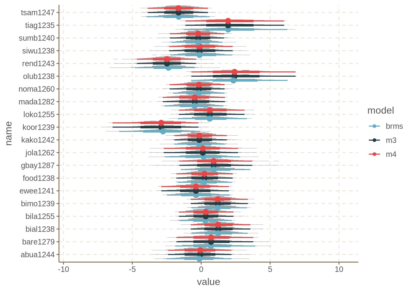
As mentioned above, both our models give identical results, while brms gives slightly different results, but pretty much on point.
One final thing to discuss is how to set the priors on the sd of the phylogentic component. This is not a simple question. In this case study I did not go into much detail on the issue and took a generic exponential(4). This is moderately regularizing (i.e. drives the coefficients closer to 0) but not much, as can be seen in the previous plot. We can explore this a bit more.
We can take the mean of the posterior of each language for the phylogenetic component. I am sorting by largest from the left and right.
group_by(s4_phylo_wide, name) %>%
  summarize(name = unique(name), value = mean(value)) %>%
  arrange(desc(value))
## # A tibble: 718 × 2
##    name     value
##    <chr>    <dbl>
##  1 ngam1268  2.69
##  2 furu1242  2.66
##  3 bagi1246  2.66
##  4 mbay1241  2.65
##  5 yulu1243  2.64
##  6 moro1284  2.61
##  7 jurm1239  2.61
##  8 baka1274  2.61
##  9 keli1248  2.59
## 10 madi1260  2.59
## # ℹ 708 more rows
group_by(s4_phylo_wide, name) %>%
  summarize(name = unique(name), value = mean(value)) %>%
  arrange((value))
## # A tibble: 718 × 2
##    name     value
##    <chr>    <dbl>
##  1 kaby1243 -3.44
##  2 tach1250 -3.43
##  3 cent2194 -3.43
##  4 tawa1286 -3.39
##  5 tama1365 -3.35
##  6 taha1241 -3.26
##  7 afit1238 -3.03
##  8 amas1236 -3.02
##  9 koor1239 -2.98
## 10 zays1236 -2.93
## # ℹ 708 more rows
This shows that some languages have very large values. Consider -3.4 in logit scaled is 0.03, and 2.69 is 0.94. This is extremely strong, because it means that if you know the tree, for these languages you can make extremely strong predictions. This is an unlikely value. When building a real world model, you should take care in picking priors for the sd which lead to values in the phylogenetic component that make sense. Sadly, there is no one-fits-all solution here.
That is basically it for this tutorial.